Detection

Vanilla Object Detection

Overview

Vanilla object detection is the simplest form of detecting objects in images. It involves sliding a window across the image and applying a classifier to determine the presence of an object. This method is often computationally expensive and inefficient, but it laid the groundwork for more advanced techniques.

Real-World Example

Imagine you want to detect cats in various images. Using vanilla object detection, you’d slide a window across every part of the image, checking if a cat is present in each window. This process repeats multiple times at different scales and aspect ratios, which can be very slow.

YOLO (You Only Look Once)

Overview

YOLO revolutionized object detection by treating it as a single regression problem, straight from image pixels to bounding box coordinates and class probabilities. Unlike sliding windows or region proposal networks, YOLO divides the image into a grid and processes the entire image in a single forward pass, making it extremely fast.

Key Steps

1. Divide the image into \( S \times S \) grid: Each grid cell is responsible for predicting a fixed number of bounding boxes.

2. Mark the center: Each cell predicts bounding boxes and confidence scores for objects whose centers fall into that cell.

3. Object detection per cell: Each cell predicts multiple bounding boxes and their associated class probabilities.

The YOLO (You Only Look Once) like approach:

• Divide the image into SxX grid.

• Mark the center of each object.

Each cell should detect an object if its center falls in it.

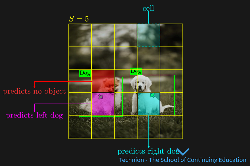
limitations

• number of object limit to S^2

• one object per cell

Real-World Example

Suppose you are building a real-time object detection system for self-driving cars. YOLO can detect various objects (like pedestrians, cars, and traffic signs) in real-time, making decisions rapidly due to its efficient architecture.

Limitations

Overview

Despite its advancements, YOLO and other object detection methods face several limitations:

1. Small Object Detection: Difficulty in detecting small objects because each grid cell predicts only a fixed number of bounding boxes.

2. Localization Errors: Sometimes less accurate in localizing the object boundaries compared to region-based methods.

3. Fixed Grid Size: Limitation in flexibility due to the fixed grid size.

Loss Function

Overview

The loss function in object detection typically combines multiple components to handle both classification and localization tasks:

1. Classification Loss: Measures how well the predicted class probabilities match the ground truth.

2. Localization Loss: Measures how well the predicted bounding boxes match the ground truth bounding boxes.

3. Confidence Loss: Measures how confident the model is about the presence of an object within a bounding box.

Mathematical Representation

The overall loss function ( L ) can be represented as:

\[ L = \lambda_{\text{coord}} L_{\text{coord}} + L_{\text{conf}} + L_{\text{class}} \]

where \( \lambda_{\text{coord}} \) is a weight factor for the localization loss \( L_{\text{coord}} \) , \( L_{\text{conf}} \) is the confidence loss, and \( L_{\text{class}} \) is the classification loss.

Anchors

Overview

Anchors are predefined bounding boxes of different sizes and aspect ratios used to handle objects of varying scales and shapes within the image. Each grid cell predicts multiple anchor boxes to accommodate multiple objects of different shapes.

Real-World Example

In a traffic surveillance system, cars, trucks, and motorcycles vary greatly in size and aspect ratio. Using anchor boxes helps the model predict bounding boxes that better fit these different objects, improving detection accuracy.

Visualization

Imagine having an image with multiple objects. Instead of predicting a single bounding box per grid cell, the model uses several anchor boxes of different shapes and sizes. This allows the detection of small objects like traffic signs and large objects like buses more accurately.