
Convolution for Frequency Estimation#
Notebook by:
Royi Avital RoyiAvital@fixelalgorithms.com
Revision History#
Version |
Date |
User |
Content / Changes |
|---|---|---|---|
1.0.000 |
29/04/2024 |
Royi Avital |
First version |
![]()
# Import Packages

# General Tools
import numpy as np
import scipy as sp
import pandas as pd

# Machine Learning
from sklearn.datasets import fetch_california_housing

# Deep Learning
import torch
import torch.nn            as nn
import torch.nn.functional as F
from torch.optim.optimizer import Optimizer
from torch.utils.data import DataLoader
from torchmetrics.regression import R2Score
import torchinfo

# Miscellaneous
import copy
import math
import os
from platform import python_version
import random
import time

# Typing
from typing import Callable, Dict, Generator, List, Optional, Self, Set, Tuple, Union

# Visualization
import matplotlib as mpl
import matplotlib.pyplot as plt
import seaborn as sns

# Jupyter
from IPython import get_ipython
from IPython.display import HTML, Image
from IPython.display import display
from ipywidgets import Dropdown, FloatSlider, interact, IntSlider, Layout, SelectionSlider
from ipywidgets import interact
Notations#
(?) Question to answer interactively.
(!) Simple task to add code for the notebook.
(@) Optional / Extra self practice.
(#) Note / Useful resource / Food for thought.
Code Notations:
someVar    = 2; #<! Notation for a variable
vVector    = np.random.rand(4) #<! Notation for 1D array
mMatrix    = np.random.rand(4, 3) #<! Notation for 2D array
tTensor    = np.random.rand(4, 3, 2, 3) #<! Notation for nD array (Tensor)
tuTuple    = (1, 2, 3) #<! Notation for a tuple
lList      = [1, 2, 3] #<! Notation for a list
dDict      = {1: 3, 2: 2, 3: 1} #<! Notation for a dictionary
oObj       = MyClass() #<! Notation for an object
dfData     = pd.DataFrame() #<! Notation for a data frame
dsData     = pd.Series() #<! Notation for a series
hObj       = plt.Axes() #<! Notation for an object / handler / function handler
Code Exercise#
Single line fill
vallToFill = ???
Multi Line to Fill (At least one)
# You need to start writing
????
Section to Fill
#===========================Fill This===========================#
# 1. Explanation about what to do.
# !! Remarks to follow / take under consideration.
mX = ???

???
#===============================================================#
# Configuration
# %matplotlib inline

seedNum = 512
np.random.seed(seedNum)
random.seed(seedNum)

# Matplotlib default color palette
lMatPltLibclr = ['#1f77b4', '#ff7f0e', '#2ca02c', '#d62728', '#9467bd', '#8c564b', '#e377c2', '#7f7f7f', '#bcbd22', '#17becf']
# sns.set_theme() #>! Apply SeaBorn theme

runInGoogleColab = 'google.colab' in str(get_ipython())

# Improve performance by benchmarking
torch.backends.cudnn.benchmark = True

# Reproducibility
# torch.manual_seed(seedNum)
# torch.backends.cudnn.deterministic = True
# torch.backends.cudnn.benchmark     = False
# Constants

FIG_SIZE_DEF    = (8, 8)
ELM_SIZE_DEF    = 50
CLASS_COLOR     = ('b', 'r')
EDGE_COLOR      = 'k'
MARKER_SIZE_DEF = 10
LINE_WIDTH_DEF  = 2

D_CLASSES_CIFAR_10  = {0: 'Airplane', 1: 'Automobile', 2: 'Bird', 3: 'Cat', 4: 'Deer', 5: 'Dog', 6: 'Frog', 7: 'Horse', 8: 'Ship', 9: 'Truck'}
L_CLASSES_CIFAR_10  = ['Airplane', 'Automobile', 'Bird', 'Cat', 'Deer', 'Dog', 'Frog', 'Horse', 'Ship', 'Truck']
T_IMG_SIZE_CIFAR_10 = (32, 32, 3)

DATA_FOLDER_PATH    = 'Data'
TENSOR_BOARD_BASE   = 'TB'
# Download Auxiliary Modules for Google Colab
if runInGoogleColab:
    !wget https://raw.githubusercontent.com/FixelAlgorithmsTeam/FixelCourses/master/AIProgram/2024_02/DataManipulation.py
    !wget https://raw.githubusercontent.com/FixelAlgorithmsTeam/FixelCourses/master/AIProgram/2024_02/DataVisualization.py
    !wget https://raw.githubusercontent.com/FixelAlgorithmsTeam/FixelCourses/master/AIProgram/2024_02/DeepLearningPyTorch.py
# Courses Packages
import sys
sys.path.append('/home/vlad/utils')
from DataVisualization import PlotRegressionResults
from DeepLearningPyTorch import NNMode, TrainModel
2024-06-03 04:39:05.743787: I tensorflow/core/platform/cpu_feature_guard.cc:182] This TensorFlow binary is optimized to use available CPU instructions in performance-critical operations.
To enable the following instructions: SSE4.1 SSE4.2 AVX AVX2 FMA, in other operations, rebuild TensorFlow with the appropriate compiler flags.
# General Auxiliary Functions

def GenHarmonicData( numSignals: int, numSamples: int, samplingFreq: float, maxFreq: float, σ: float ) -> Tuple[torch.Tensor, torch.Tensor]:

    π = np.pi #<! Constant Pi

    vT   = torch.linspace(0, numSamples - 1, numSamples) / samplingFreq #<! Time samples
    vF   = maxFreq * torch.rand(numSignals)                             #<! Frequency per signal
    vPhi = 2 * π * torch.rand(numSignals)                               #<! Phase per signal

    # x_i(t) = sin(2π f_i t + φ_i) + n_i(t)
    mX = torch.sin(2 * π * vF[:, None] @ vT[None, :] + vPhi[:, None])       ## @ is matrix multiplication in PyTorch
    mX = mX + σ * torch.randn(mX.shape) #<! Add noise

    return mX, vF
Frequency Estimation with 1D Convolution Model in PyTorch#
This notebook estimates the frequency of a given set of samples of an Harmonic Signal.
The notebook presents:
Use of convolution layers in PyTorch.
Use of pool layers in PyTorch.
Use of adaptive pool layer in PyTorch.
The motivation is to set a constant output size regardless of input.Use the model for inference on the test data.
(#) While the layers are called Convolution Layer they actually implement correlation.
Since the weights are learned, in practice it makes no difference as Correlation is convolution with the a flipped kernel.
(?) What kind of a problem it frequency estimation? - regression!
# Parameters

# Data
numSignalsTrain = 15_000
numSignalsVal   = 5_000
numSignalsTest  = 5_000

numSamples = 500 #<! Samples in Signal

maxFreq      = 10.0  #<! [Hz]
samplingFreq = 100.0 #<! [Hz]

σ      = 0.1 #<! Noise Std

# Model
dropP = 0.1 #<! Dropout Layer

# Training
batchSize   = 256
numWork     = 2 #<! Number of workers
nEpochs     = 20

# Visualization
numSigPlot = 5
Generate / Load Data#
This section generates the data from the following model:
\(\boldsymbol{x}_{i}\) - Set of input samples (
numSamples) of the \(i\) -th Harmonic Signal.\({f}_{i}\) - The signal frequency in the range
[0, maxFreq].\(t\) - Time sample.
\(\phi_{i}\) - The signal phase in the range
[0, 2π].\(\boldsymbol{n}_{i}\) - Set of noise samples (
numSamples) of the \(i\) -th Harmonic Signal.
The noise standard deviation is set toσ.
The model input data is in the format: \({N}_{b} \times {C} \times N\):
\({N}_{b}\) - Number of signals in the batch (
batchSize).\(C\) - Number of channels (The signal is a single channel).
(#) Since it is a generated data set, data can be generated at will.
(#) The signal 1D with a single channel. EEG signals, Stereo Audio signal, ECG signals are examples for multi channel 1D signals.
The concept of 1D in this context is the index which the data is generated along.
# Generate Data

mXTrain, vYTrain    = GenHarmonicData(numSignalsTrain, numSamples, samplingFreq, maxFreq, σ) #<! Train Data
mXVal, vYVal        = GenHarmonicData(numSignalsVal, numSamples, samplingFreq, maxFreq, σ)   #<! Validation Data
mXTest, vYTest      = GenHarmonicData(numSignalsTest, numSamples, samplingFreq, maxFreq, σ)  #<! Test Data

vT = np.linspace(0, numSamples - 1, numSamples) / samplingFreq #<! For plotting

mX = torch.concatenate((mXTrain, mXVal), axis = 0)
vY = torch.concatenate((vYTrain, vYVal), axis = 0)

print(f'The features data shape: {mX.shape}')
print(f'The labels data shape: {vY.shape}')
The features data shape: torch.Size([20000, 500])
The labels data shape: torch.Size([20000])
(?) What is the content of
vYabove? Explain its shape.
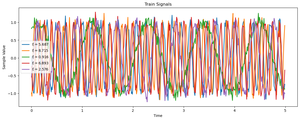
Plot Data#
# Plot the Data

hF, hA = plt.subplots(figsize = (14, 5))
for _ in range(numSigPlot):
    idxSig = np.random.randint(numSignalsTrain)
    vX  = mXTrain[idxSig,:]
    hA.plot(vT, vX, lw = 2, label = f'$f_i = {(vYTrain[idxSig].item()):.3f}$')

hA.set_title('Train Signals')
hA.set_xlabel('Time')
hA.set_ylabel('Sample Value')
hA.legend()
plt.show()
print(f"mXTrain.shape = {mXTrain.shape}")
print(f"vXType = {type(mXTrain)}")

print(f'converted view shape {mXTrain.view(numSignalsTrain, 1, -1).shape}')
mXTrain.shape = torch.Size([15000, 500])
vXType = <class 'torch.Tensor'>
converted view shape torch.Size([15000, 1, 500])
help view:
|  view(...)
|      view(*shape) -> Tensor
|
|      Returns a new tensor with the same data as the :attr:`self` tensor but of a
|      different :attr:`shape`.
|
|      The returned tensor shares the same data and must have the same number
|      of elements, but may have a different size. For a tensor to be viewed, the new
|      view size must be compatible with its original size and stride, i.e., each new
|      view dimension must either be a subspace of an original dimension, or only span
|      across original dimensions :math:`d, d+1, \dots, d+k` that satisfy the following
|      contiguity-like condition that :math:`\forall i = d, \dots, d+k-1`,
|
|      .. math::
|
|        \text{stride}[i] = \text{stride}[i+1] \times \text{size}[i+1]
|
|      Otherwise, it will not be possible to view :attr:`self` tensor as :attr:`shape`
|      without copying it (e.g., via :meth:`contiguous`). When it is unclear whether a
|      :meth:`view` can be performed, it is advisable to use :meth:`reshape`, which
|      returns a view if the shapes are compatible, and copies (equivalent to calling
|      :meth:`contiguous`) otherwise.
|
|      Args:
|          shape (torch.Size or int...): the desired size
|
|      Example::
|
|          >>> x = torch.randn(4, 4)
|          >>> x.size()
|          torch.Size([4, 4])
|          >>> y = x.view(16)
|          >>> y.size()
|          torch.Size([16])
|          >>> z = x.view(-1, 8)  # the size -1 is inferred from other dimensions
|          >>> z.size()
|          torch.Size([2, 8])
Input Data#
There are several ways to convert the data into the shape expected by the model convention:
# Assume: mX.shape = (N, L)
mX = mX.view(N, 1, L) #<! Option I
mX = mX.unsqueeze(1)  #<! Option II
mX = mX[:, None, :]   #<! Option III
#Output: mX.shape = (N, 1, L)
# Data Sets

dsTrain = torch.utils.data.TensorDataset(mXTrain.view(numSignalsTrain, 1, -1), vYTrain) #<! -1 -> Infer
dsVal   = torch.utils.data.TensorDataset(mXVal.view(numSignalsVal, 1, -1), vYVal)
dsTest  = torch.utils.data.TensorDataset(mXTest.view(numSignalsTest, 1, -1), vYTest)
(?) Does the data require standardization? Why?
– no need the data is generated with the same scale in 0-1 range.
# Data Loaders

# Data is small, no real need for workers
dlTrain  = torch.utils.data.DataLoader(dsTrain, shuffle = True, batch_size = 1 * batchSize, num_workers = numWork, persistent_workers = True)
dlTest   = torch.utils.data.DataLoader(dsTest, shuffle = False, batch_size = 2 * batchSize, num_workers = numWork, persistent_workers = True)
# Iterate on the Loader
# The first batch.
tX, vY = next(iter(dlTrain)) #<! PyTorch Tensors

print(f'The batch features dimensions: {tX.shape}')
print(f'The batch labels dimensions: {vY.shape}')
The batch features dimensions: torch.Size([256, 1, 500])
The batch labels dimensions: torch.Size([256])
Define the Model#
The model is defined as a sequential model.
# Model
# Defining a sequential model.

numFeatures = mX.shape[1]

def GetModel( ) -> nn.Module:
    oModel = nn.Sequential(
        nn.Identity(),

        nn.Conv1d(in_channels = 1,   out_channels = 32,  kernel_size = 11), nn.MaxPool1d(kernel_size = 2), nn.ReLU(),
        nn.Conv1d(in_channels = 32,  out_channels = 64,  kernel_size = 11), nn.MaxPool1d(kernel_size = 2), nn.ReLU(),
        nn.Conv1d(in_channels = 64,  out_channels = 128, kernel_size = 11), nn.MaxPool1d(kernel_size = 2), nn.ReLU(),
        nn.Conv1d(in_channels = 128, out_channels = 256, kernel_size = 11), nn.MaxPool1d(kernel_size = 2), nn.ReLU(),

        nn.AdaptiveAvgPool1d(output_size = 1),
        nn.Flatten          (),
        nn.Linear           (in_features = 256, out_features = 1),
        nn.Flatten          (start_dim = 0),
        )

    return oModel
layer1:
==========

cin =1  cout = 32   size=11

32*11 + 32 = 384


adaptive avg pool1d:
====================

input was (256 256 21)
then that block just average that to 1 dim : (256 256 1)
(#) The
torch.nn.AdaptiveAvgPool1dallows the same output shape regard less of the input.(?) What is the role of the
torch.nn.Flattenlayers?
# Model Summary

oModel = GetModel()
torchinfo.summary(oModel, tX.shape, device = 'cpu')
==========================================================================================
Layer (type:depth-idx)                   Output Shape              Param #
==========================================================================================
Sequential                               [256]                     --
├─Identity: 1-1                          [256, 1, 500]             --
├─Conv1d: 1-2                            [256, 32, 490]            384
├─MaxPool1d: 1-3                         [256, 32, 245]            --
├─ReLU: 1-4                              [256, 32, 245]            --
├─Conv1d: 1-5                            [256, 64, 235]            22,592
├─MaxPool1d: 1-6                         [256, 64, 117]            --
├─ReLU: 1-7                              [256, 64, 117]            --
├─Conv1d: 1-8                            [256, 128, 107]           90,240
├─MaxPool1d: 1-9                         [256, 128, 53]            --
├─ReLU: 1-10                             [256, 128, 53]            --
├─Conv1d: 1-11                           [256, 256, 43]            360,704
├─MaxPool1d: 1-12                        [256, 256, 21]            --
├─ReLU: 1-13                             [256, 256, 21]            --
├─AdaptiveAvgPool1d: 1-14                [256, 256, 1]             --
├─Flatten: 1-15                          [256, 256]                --
├─Linear: 1-16                           [256, 1]                  257
├─Flatten: 1-17                          [256]                     --
==========================================================================================
Total params: 474,177
Trainable params: 474,177
Non-trainable params: 0
Total mult-adds (Units.GIGABYTES): 7.85
==========================================================================================
Input size (MB): 0.51
Forward/backward pass size (MB): 113.51
Params size (MB): 1.90
Estimated Total Size (MB): 115.92
==========================================================================================
(#) Pay attention the dropout parameter of PyTorch is about the probability to zero out the value.
# Run Model
# Apply a test run.

mXX = torch.randn(batchSize, numSamples)
mXX = mXX.view(batchSize, 1, numSamples)
with torch.inference_mode():
    vYHat = oModel(mXX)

print(f'The input dimensions: {mXX.shape}')
print(f'The output dimensions: {vYHat.shape}')
The input dimensions: torch.Size([256, 1, 500])
The output dimensions: torch.Size([256])
Training Loop#
Use the training and validation samples.
The objective will be defined as the Mean Squared Error and the score as \({R}^{2}\).
(?) Will the best model loss wise will be the model with the best score? Explain specifically and generally (For other loss and scores).
– not necessarily, the loss is the difference between the predicted value and the true value, while the score is the correlation between the predicted value and the true value.
Train the Model#
# Check GPU Availability

runDevice   = torch.device('cuda:0' if torch.cuda.is_available() else 'cpu') #<! The 1st CUDA device
oModel      = oModel.to(runDevice) #<! Transfer model to device
# Set the Loss & Score

hL = nn.MSELoss()
hS = R2Score(num_outputs = 1)
hS = hS.to(runDevice)
# Define Optimizer

oOpt = torch.optim.AdamW(oModel.parameters(), lr = 1e-4, betas = (0.9, 0.99), weight_decay = 1e-5) #<! Define optimizer
# Train the Model

oRunModel, lTrainLoss, lTrainScore, lValLoss, lValScore, _ = TrainModel(oModel, dlTrain, dlTest, oOpt, nEpochs, hL, hS)
Epoch    1 / 20 | Train Loss: 11.911 | Val Loss:  1.082 | Train Score: -0.425 | Val Score:  0.870 | Epoch Time: 18.70 | <-- Checkpoint! |
Epoch    2 / 20 | Train Loss:  0.358 | Val Loss:  0.107 | Train Score:  0.957 | Val Score:  0.987 | Epoch Time:  1.82 | <-- Checkpoint! |
Epoch    3 / 20 | Train Loss:  0.054 | Val Loss:  0.021 | Train Score:  0.994 | Val Score:  0.998 | Epoch Time:  1.83 | <-- Checkpoint! |
Epoch    4 / 20 | Train Loss:  0.013 | Val Loss:  0.008 | Train Score:  0.998 | Val Score:  0.999 | Epoch Time:  1.81 | <-- Checkpoint! |
Epoch    5 / 20 | Train Loss:  0.007 | Val Loss:  0.007 | Train Score:  0.999 | Val Score:  0.999 | Epoch Time:  1.80 | <-- Checkpoint! |
Epoch    6 / 20 | Train Loss:  0.005 | Val Loss:  0.005 | Train Score:  0.999 | Val Score:  0.999 | Epoch Time:  1.81 | <-- Checkpoint! |
Epoch    7 / 20 | Train Loss:  0.004 | Val Loss:  0.005 | Train Score:  0.999 | Val Score:  0.999 | Epoch Time:  1.85 | <-- Checkpoint! |
Epoch    8 / 20 | Train Loss:  0.004 | Val Loss:  0.004 | Train Score:  0.999 | Val Score:  0.999 | Epoch Time:  1.80 | <-- Checkpoint! |
Epoch    9 / 20 | Train Loss:  0.004 | Val Loss:  0.004 | Train Score:  1.000 | Val Score:  1.000 | Epoch Time:  1.89 | <-- Checkpoint! |
Epoch   10 / 20 | Train Loss:  0.004 | Val Loss:  0.004 | Train Score:  1.000 | Val Score:  0.999 | Epoch Time:  1.80 |
Epoch   11 / 20 | Train Loss:  0.004 | Val Loss:  0.004 | Train Score:  1.000 | Val Score:  1.000 | Epoch Time:  1.81 | <-- Checkpoint! |
Epoch   12 / 20 | Train Loss:  0.004 | Val Loss:  0.004 | Train Score:  1.000 | Val Score:  1.000 | Epoch Time:  1.81 |
Epoch   13 / 20 | Train Loss:  0.004 | Val Loss:  0.004 | Train Score:  1.000 | Val Score:  1.000 | Epoch Time:  1.80 | <-- Checkpoint! |
Epoch   14 / 20 | Train Loss:  0.004 | Val Loss:  0.004 | Train Score:  1.000 | Val Score:  1.000 | Epoch Time:  1.80 |
Epoch   15 / 20 | Train Loss:  0.004 | Val Loss:  0.003 | Train Score:  1.000 | Val Score:  1.000 | Epoch Time:  1.79 | <-- Checkpoint! |
Epoch   16 / 20 | Train Loss:  0.003 | Val Loss:  0.003 | Train Score:  1.000 | Val Score:  1.000 | Epoch Time:  1.81 | <-- Checkpoint! |
Epoch   17 / 20 | Train Loss:  0.004 | Val Loss:  0.004 | Train Score:  1.000 | Val Score:  1.000 | Epoch Time:  1.81 |
Epoch   18 / 20 | Train Loss:  0.003 | Val Loss:  0.003 | Train Score:  1.000 | Val Score:  1.000 | Epoch Time:  1.83 | <-- Checkpoint! |
Epoch   19 / 20 | Train Loss:  0.003 | Val Loss:  0.003 | Train Score:  1.000 | Val Score:  1.000 | Epoch Time:  1.83 | <-- Checkpoint! |
Epoch   20 / 20 | Train Loss:  0.003 | Val Loss:  0.004 | Train Score:  1.000 | Val Score:  1.000 | Epoch Time:  1.83 |
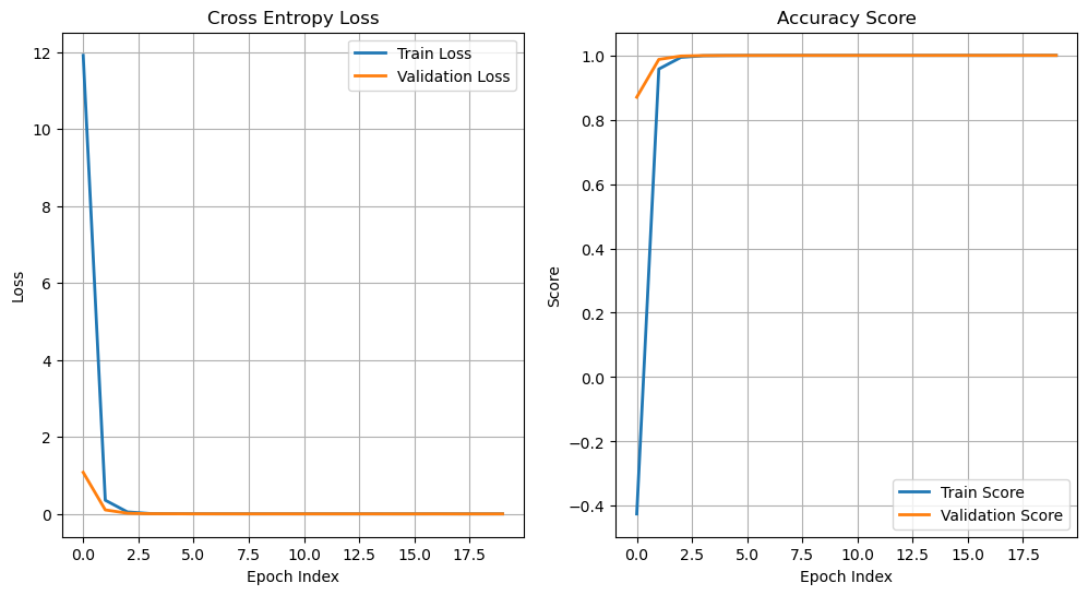
# Plot Results
hF, vHa = plt.subplots(nrows = 1, ncols = 2, figsize = (12, 6))
vHa = vHa.flat

hA = vHa[0]
hA.plot(lTrainLoss, lw = 2, label = 'Train Loss')
hA.plot(lValLoss, lw = 2, label = 'Validation Loss')
hA.grid()
hA.set_title('Cross Entropy Loss')
hA.set_xlabel('Epoch Index')
hA.set_ylabel('Loss')
hA.legend();


hA = vHa[1]
hA.plot(lTrainScore, lw = 2, label = 'Train Score')
hA.plot(lValScore, lw = 2, label = 'Validation Score')
hA.grid()
hA.set_title('Accuracy Score')
hA.set_xlabel('Epoch Index')
hA.set_ylabel('Score')
hA.legend();
Test Data Analysis#
This section runs the model on the test data and analyze results.
Test Data Results#
# Run on Test Data
lYY     = []
lYYHat  = []
with torch.inference_mode():
    for tXX, vYY in dlTest:
        tXX = tXX.to(runDevice)
        lYY.append(vYY)
        lYYHat.append(oModel(tXX))

vYY    = torch.cat(lYY, dim = 0).cpu().numpy()
vYYHat = torch.cat(lYYHat, dim = 0).cpu().numpy()
(#) One could run the above using
mXTest.
The motivation is to show the general way which can handle large data set.
# Plot Regression Result

# Plot the Data

scoreR2 = hS(torch.tensor(vYY), torch.tensor(vYYHat))

hF, hA = plt.subplots(figsize = (14, 5))
hA = PlotRegressionResults(vYY, vYYHat, hA = hA)
hA.set_title(f'Test Data Set, R2 = {scoreR2:0.2f}')
hA.grid()
hA.set_xlabel('Input Frequency')
hA.set_ylabel('Estimated Frequency')

plt.show()
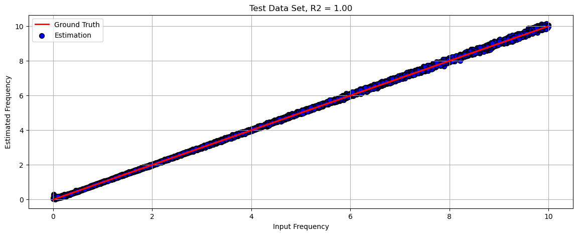
(?) Can you find where the model struggles?
(?) Can it handle shorter signals? For examples 200 samples. How?
(?) How will it generalize to cases with frequency above
maxFreq?
Extended Test Set#
This section shows the performance of the model on data with frequencies spanned on the range [0, 2 * maxFreq].
# Generate Data

mXTest, vYTest = GenHarmonicData(numSignalsTest, numSamples, samplingFreq, 2 * maxFreq, σ)  #<! Test Data
# Run on Test Data

with torch.inference_mode():
    vYTestHat = oModel(mXTest.view(numSignalsTest, 1, -1).to(runDevice))

vYTestHat = vYTestHat.cpu()
# Plot Regression Result

# Plot the Data

scoreR2 = hS(vYTest, vYTestHat)

hF, hA = plt.subplots(figsize = (14, 5))
hA = PlotRegressionResults(vYTest.cpu().numpy(), vYTestHat.cpu().numpy(), hA = hA)
hA.set_title(f'Test Data Set, R2 = {scoreR2:0.2f}')
hA.grid()
hA.set_xlabel('Input Frequency')
hA.set_ylabel('Estimated Frequency')

plt.show()
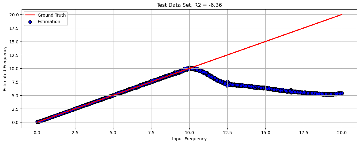
(?) Why does the model perform poorly?
the network didnt learned the frequency; אין הכללה
(#) DL models do extrapolate and able to generalize (Think model which plays Chess).
Yet in order to generalize, the model loss and architecture has to built accordingly.
For most common cases, one must validate the train set matches the production data.