MNIST KNN

Notebook by:

• Royi Avital RoyiAvital@fixelalgorithms.com

Revision History

Version	Date	User	Content / Changes
1.0.000	10/03/2024	Royi Avital	First version

# Import Packages

# General Tools
import numpy as np
import scipy as sp
import pandas as pd

# Machine Learning
from sklearn.datasets import fetch_openml
from sklearn.metrics import confusion_matrix, ConfusionMatrixDisplay
from sklearn.model_selection import cross_val_predict, KFold, StratifiedKFold, train_test_split
from sklearn.neighbors import KNeighborsClassifier

# Image Processing

# Machine Learning

# Miscellaneous
import math
import os
from platform import python_version
import random
import timeit

# Typing
from typing import Callable, Dict, List, Optional, Set, Tuple, Union

# Visualization
import matplotlib as mpl
import matplotlib.pyplot as plt
import seaborn as sns

# Jupyter
from IPython import get_ipython
from IPython.display import Image
from IPython.display import display
from ipywidgets import Dropdown, FloatSlider, interact, IntSlider, Layout, SelectionSlider
from ipywidgets import interact

Notations

• (?) Question to answer interactively.

• (!) Simple task to add code for the notebook.

• (@) Optional / Extra self practice.

• (#) Note / Useful resource / Food for thought.

Code Notations:

someVar    = 2; #<! Notation for a variable
vVector    = np.random.rand(4) #<! Notation for 1D array
mMatrix    = np.random.rand(4, 3) #<! Notation for 2D array
tTensor    = np.random.rand(4, 3, 2, 3) #<! Notation for nD array (Tensor)
tuTuple    = (1, 2, 3) #<! Notation for a tuple
lList      = [1, 2, 3] #<! Notation for a list
dDict      = {1: 3, 2: 2, 3: 1} #<! Notation for a dictionary
oObj       = MyClass() #<! Notation for an object
dfData     = pd.DataFrame() #<! Notation for a data frame
dsData     = pd.Series() #<! Notation for a series
hObj       = plt.Axes() #<! Notation for an object / handler / function handler

Code Exercise

• Single line fill

vallToFill = ???

• Multi Line to Fill (At least one)

# You need to start writing
????

• Section to Fill

#===========================Fill This===========================#
# 1. Explanation about what to do.
# !! Remarks to follow / take under consideration.
mX = ???

???
#===============================================================#

# Configuration
# %matplotlib inline

seedNum = 512
np.random.seed(seedNum)
random.seed(seedNum)

# Matplotlib default color palette
lMatPltLibclr = ['#1f77b4', '#ff7f0e', '#2ca02c', '#d62728', '#9467bd', '#8c564b', '#e377c2', '#7f7f7f', '#bcbd22', '#17becf']
# sns.set_theme() #>! Apply SeaBorn theme

runInGoogleColab = 'google.colab' in str(get_ipython())

# Constants

FIG_SIZE_DEF    = (8, 8)
ELM_SIZE_DEF    = 50
CLASS_COLOR     = ('b', 'r')
EDGE_COLOR      = 'k'
MARKER_SIZE_DEF = 10
LINE_WIDTH_DEF  = 2

# Courses Packages
import sys
sys.path.append('../')
sys.path.append('../../')
sys.path.append('../../../')
from utils.DataVisualization import PlotConfusionMatrix, PlotLabelsHistogram, PlotMnistImages

# General Auxiliary Functions

# Parameters

# Data Generation
numImg  = 3
vSize   = [28, 28] #<! Size of images

numSamples  = 10_000
trainRatio  = 0.55
testRatio   = 1 - trainRatio


# Data Visualization

Generate / Load Data

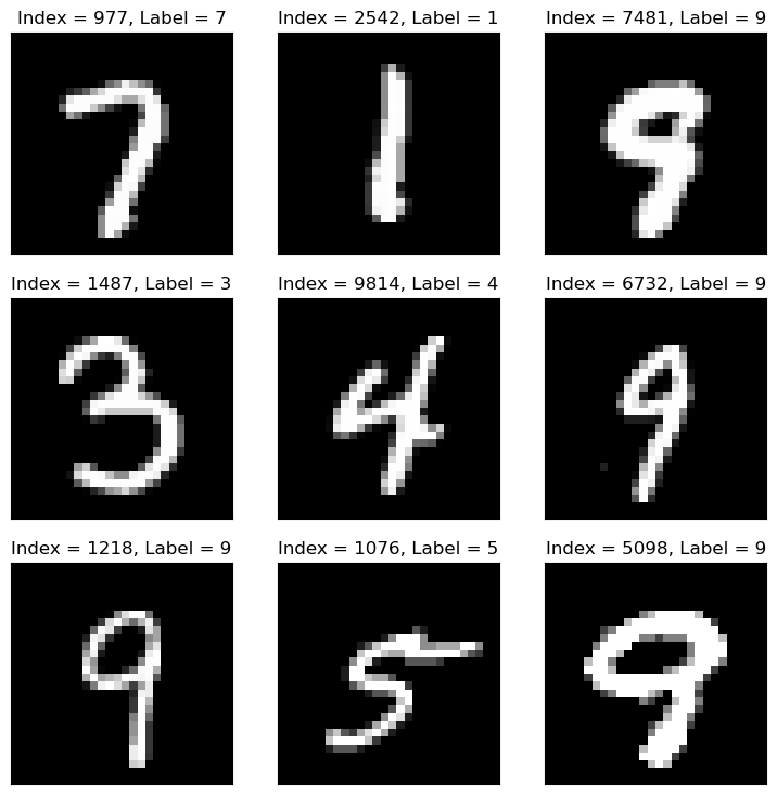
The MNIST database (Modified National Institute of Standards and Technology database) is a large database of handwritten digits.
The MNIST data is a well known data set in Machine Learning, basically it is the Hello World of ML.

The original black and white images from NIST were normalized to fit into a 28x28 pixel bounding box and anti aliased.

• (#) There is an extended version called EMNIST.

# Load Data 

mX, vY = fetch_openml('mnist_784', version = 1, return_X_y = True, as_frame = False, parser = 'auto')
vY = vY.astype(np.int_) #<! The labels are strings, convert to integer

print(f'The features data shape: {mX.shape}')
print(f'The labels data shape: {vY.shape}')
print(f'The unique values of the labels: {np.unique(vY)}')

The features data shape: (70000, 784)
The labels data shape: (70000,)
The unique values of the labels: [0 1 2 3 4 5 6 7 8 9]

# Pre Process Data
# Scaling the data values.

# The image is in the range {0, 1, ..., 255}
# We scale it into [0, 1]

mX = mX / 255

• (#) Try to do the scaling with mX /= 255.0. It will fail, try to understand why.

# Data Sub Sampling
# The data has many samples, for fast run time we'll sub sample it

vSampleIdx = np.random.choice(mX.shape[0], numSamples, replace = False)
mX = mX[vSampleIdx, :]
vY = vY[vSampleIdx]

print(f'The features data shape: {mX.shape}')
print(f'The labels data shape: {vY.shape}')
print(f'The unique values of the labels: {np.unique(vY)}')

The features data shape: (10000, 784)
The labels data shape: (10000,)
The unique values of the labels: [0 1 2 3 4 5 6 7 8 9]

Plot Data

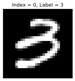
# Plot the Data

hF = PlotMnistImages(mX, vY, numImg)

Distribution of Labels

When dealing with classification, it is important to know the balance between the labels within the data set.

# Distribution of Labels

hA = PlotLabelsHistogram(vY)
plt.show()

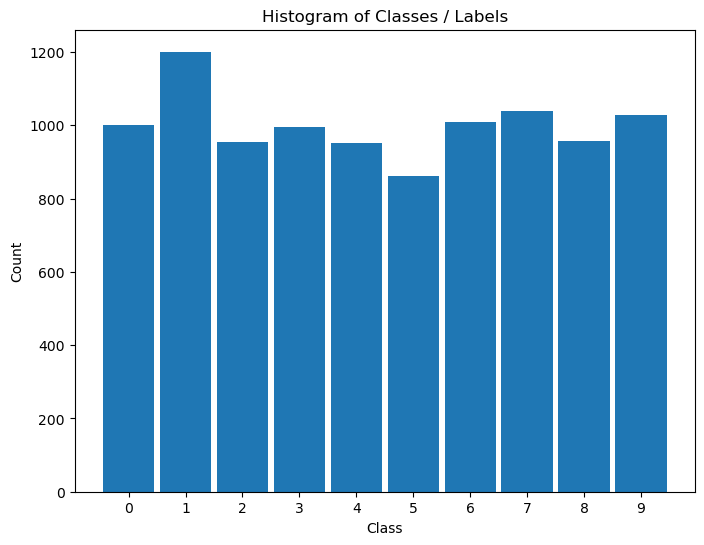
• (?) Looking at the histogram of labels, Is the data balanced?

Train / Test Split

In this section we’ll split the data into 2 sub sets: Train and Test.

• (?) The split will be random. What could be the issue with that? Think of the balance of labels.

# Train & Test Split
# SciKit Learn has a built in tool for this split.
# It can take ratios or integer numbers.
# In case only `train_size` or `test_size` is given the other one is the rest of the data.
mXTrain, mXTest, vYTrain, vYTest = train_test_split(mX, vY, train_size = trainRatio, test_size = testRatio, random_state = seedNum)

print(f"for trainRatio = {trainRatio} the testRatio = {testRatio}")
print(f'The train features data shape: {mXTrain.shape}')
print(f'The train labels data shape: {vYTrain.shape}')
print(f'The test features data shape: {mXTest.shape}')
print(f'The test labels data shape: {vYTest.shape}')

for trainRatio = 0.55 the testRatio = 0.44999999999999996
The train features data shape: (5500, 784)
The train labels data shape: (5500,)
The test features data shape: (4500, 784)
The test labels data shape: (4500,)

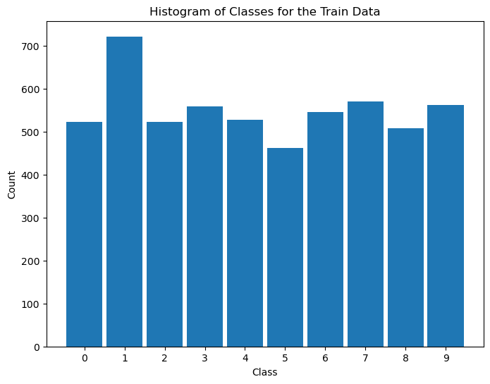
# Distribution of Labels (Train)
# Distribution of classes in train data.

hA = PlotLabelsHistogram(vYTrain)
hA.set_title('Histogram of Classes for the Train Data')
plt.show()

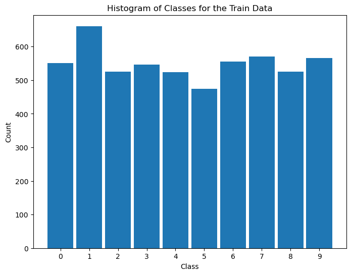
use stratify:

mXTrain, mXTest, vYTrain, vYTest = train_test_split(mX, vY, train_size = trainRatio, test_size = testRatio, random_state = seedNum,stratify=vY)

print(f"for trainRatio = {trainRatio} the testRatio = {testRatio}")
print(f'The train features data shape: {mXTrain.shape}')
print(f'The train labels data shape: {vYTrain.shape}')
print(f'The test features data shape: {mXTest.shape}')
print(f'The test labels data shape: {vYTest.shape}')

for trainRatio = 0.55 the testRatio = 0.44999999999999996
The train features data shape: (5500, 784)
The train labels data shape: (5500,)
The test features data shape: (4500, 784)
The test labels data shape: (4500,)

# Distribution of Labels (Train)
# Distribution of classes in train data.

hA = PlotLabelsHistogram(vYTrain)
hA.set_title('Histogram of Classes for the Train Data')
plt.show()

# Distribution of Labels (Test)
# Distribution of classes in test data.

hA = PlotLabelsHistogram(vYTest)
hA.set_title('Histogram of Classes for the Test Data')
plt.show()

• (?) Do you see the same distribution at both sets? What does it mean?

• (!) Use the stratify option in train_test_split() and look at the results.

Train a K-NN Model

In this section we’ll train a K-NN model on the train data set and test its performance on the test data set.

# K-NN Model
K = 1
oKnnCls = KNeighborsClassifier(n_neighbors = K)
oKnnCls = oKnnCls.fit(mXTrain, vYTrain)

(?) What would be the score on the train set?
(?) What would be the relation between the performance on the train set vs. test set?

# Prediction on the Train Set

rndIdx  = np.random.randint(mXTrain.shape[0])

## predict in scikit learn need a 2d array !!!!!!!!!!!!!!!!!!!!!!!!!!!!!!!!!!!!!!!!!!!!!!! => use atleast_2d !!!
yPred = oKnnCls.predict(np.atleast_2d(mXTrain[rndIdx, :])) #<! The input must be 2D data


hF = PlotMnistImages(np.atleast_2d(mXTrain[rndIdx, :]), yPred, 1)

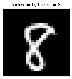
# Prediction on the Test Set

rndIdx  = np.random.randint(mXTest.shape[0])
yPred = oKnnCls.predict(np.atleast_2d(mXTest[rndIdx, :])) #<! The input must be 2D data
hF = PlotMnistImages(np.atleast_2d(mXTest[rndIdx, :]), yPred, 1)

• (!) Find the sample in the train data set which is closest to the sample above.

Confusion Matrix and Score on Train and Test Sets

In this section we’ll evaluate the performance of the model on the train and test sets.
The SciKit Learn package has some built in functions / classes to display those: confusion_matrix(), ConfusionMatrixDisplay.

# Predictions
# Computing the prediction per set.
vYTrainPred = oKnnCls.predict(mXTrain) #<! Predict train set
vYTestPred  = oKnnCls.predict(mXTest)  #<! Predict test set

trainAcc = oKnnCls.score(mXTrain, vYTrain)
testAcc  = oKnnCls.score(mXTest, vYTest)

# Plot the Confusion Matrix

hF, hA = plt.subplots(nrows = 1, ncols = 2, figsize = (14, 6)) #<! Figure

# Arranging data for the plot function
lConfMatData = [{'vY': vYTrain, 'vYPred': vYTrainPred, 'hA': hA[0], 'dScore': {'Accuracy': trainAcc}, 'titleStr': 'Train - Confusion Matrix'},
{'vY': vYTest, 'vYPred': vYTestPred, 'hA': hA[1], 'dScore': {'Accuracy': testAcc}, 'titleStr': 'Test - Confusion Matrix'}]

for ii in range(2):
    PlotConfusionMatrix(**lConfMatData[ii])

plt.show()

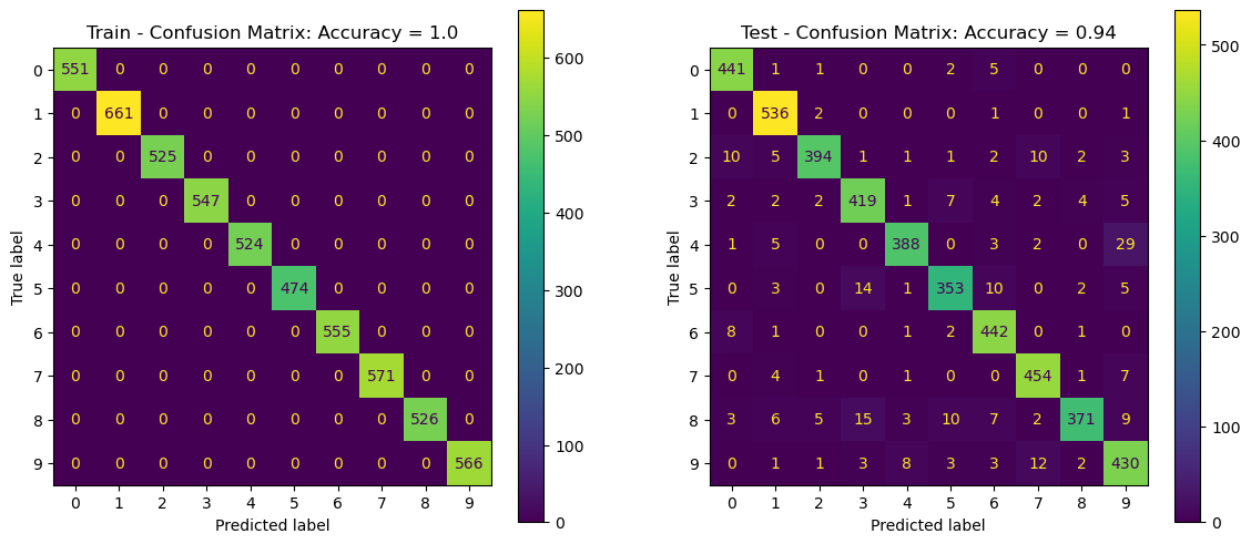
• (?) Look at the most probable error per label, does it make sense?

• (?) What do you expect to happen with a different K?

• (!) Run the above with different values of K. => plot graph on K till 20…

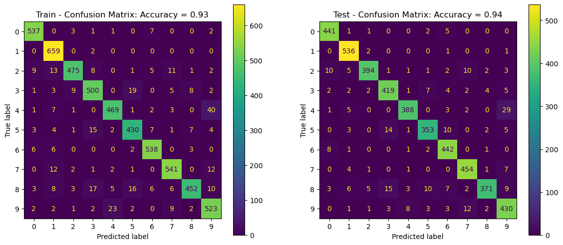
Cross Validation

The Cross Validation process allows us to estimate the stability of performance.
It also the main tool to optimize the model Hyper Parameters.

Cross Validation as a Measure of Test Performance

Let’s see if indeed the cross validation is a better way to estimate the performance of the test set.
We can do that using Cross Validation on the training set. We’ll predict the label of each sample using other data. We’ll use a K-Fold Cross Validation with stratified option to keep the data distribution in tact.

# Cross Validation & Predict
# Prediction the classes using Cross Validation.
numFold = 10

vYTrainPred = cross_val_predict(KNeighborsClassifier(n_neighbors = K), mXTrain, vYTrain, cv = KFold(numFold, shuffle = True))
trainAcc = np.mean(vYTrainPred == vYTrain)

• (!) Change the values of numFold. Try extreme values. What happens?

• (@) Repeat the above with StratifiedKFold().

# Plot the Confusion Matrix

hF, hA = plt.subplots(nrows = 1, ncols = 2, figsize = (14, 6)) #<! Figure

# Arranging data for the plot function
lConfMatData = [{'vY': vYTrain, 'vYPred': vYTrainPred, 'hA': hA[0], 'dScore': {'Accuracy': trainAcc}, 'titleStr': 'Train - Confusion Matrix'},
{'vY': vYTest, 'vYPred': vYTestPred, 'hA': hA[1], 'dScore': {'Accuracy': testAcc}, 'titleStr': 'Test - Confusion Matrix'}]

for ii in range(2):
    PlotConfusionMatrix(**lConfMatData[ii])

plt.show()

• (!) Use the normMethod parameter to normalize the confusion matrix by rows, columns or all.

Cross Validation for Hyper Parameter Optimization

We can also use the Cross Validation approach to search for the best Hype Parameter.
The idea is iterating through the data and measure the score we care about.
The hyper parameter which maximize the score will be used for the production model.

• (#) Usually, once we set the optimal hyper parameters we’ll re train the model on the whole data set.

• (#) We’ll learn how to to automate this process later using built in tools, but the idea is the same.

# Cross Validation for the K parameters
numFold = 10

lK = list(range(1, 13, 2)) #<! Range of values of K
print(f'The range of K: {lK}')
numK = len(lK)

lAcc = [None] * numK

for ii, K in enumerate(lK):
    vYTrainPred = cross_val_predict(KNeighborsClassifier(n_neighbors = K), mX, vY, cv = StratifiedKFold(numFold, shuffle = True))
    lAcc[ii] = np.mean(vYTrainPred == vY)  ## accuracy

The range of K: [1, 3, 5, 7, 9, 11]

# Plot Results

hF, hA = plt.subplots(figsize = FIG_SIZE_DEF)
hA.plot(lK, lAcc)
hA.scatter(lK, lAcc, s = 100)
hA.set_title('Accuracy Score as a Function of K')
hA.set_xlabel('K')
hA.set_ylabel('Accuracy')
hA.set_xticks(lK)
hA.grid()

plt.show()

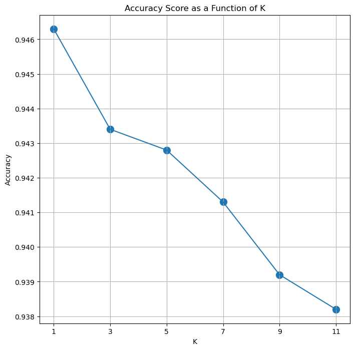
• (?) What’s the optimal K?

• (?) What’s the Dynamic Range of the results? Think again on the question above.