Mahalanobis

Mahalanobis Distance for Anomaly Detection

General Overview

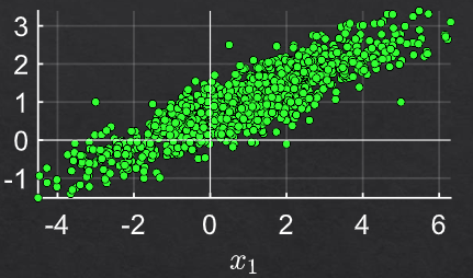
The Mahalanobis distance is a measure of the distance between a point and a distribution. Unlike the Euclidean distance, which simply measures the straight-line distance between two points, the Mahalanobis distance accounts for the correlations between variables in a dataset. This makes it particularly useful for identifying outliers in multivariate data.

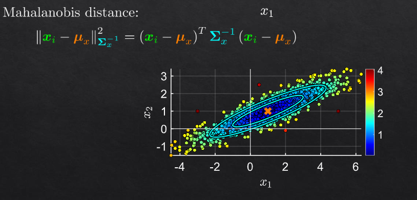
The Mahalanobis distance of a vector \( \mathbf{x} \) from a distribution with mean \( \mu \) and covariance matrix \( \Sigma \) is given by:

\[ D_M(\mathbf{x}) = \sqrt{(\mathbf{x} - \mathbf{\mu})^T \Sigma^{-1} (\mathbf{x} - \mathbf{\mu})} \]

where:

• \( \mathbf{x} \) is the data point,

• \( \mathbf{\mu} \) is the mean vector of the distribution,

• \( \Sigma \) is the covariance matrix of the distribution,

• \( \Sigma^{-1} \) is the inverse of the covariance matrix.

Real-World Examples

1. Credit Risk Analysis: In finance, the Mahalanobis distance can be used to identify unusual patterns in credit applications. For example, if most applicants have similar income, debt, and credit score profiles, an application that significantly deviates from this profile could be flagged for further review.

2. Industrial Quality Control: In manufacturing, this distance can help identify defective products. If the features of a product (e.g., dimensions, weight) significantly deviate from the standard, it could indicate a production issue.

3. Healthcare Diagnostics: In medical diagnostics, the Mahalanobis distance can be used to identify patients whose test results deviate significantly from the norm, potentially indicating a rare disease or condition.

Example Calculation

Consider a dataset of three-dimensional data points representing different features (e.g., height, weight, age) of individuals:

\[\begin{split} \mathbf{X} = \begin{pmatrix} 65 & 70 & 68 \\ 150 & 160 & 155 \\ 30 & 35 & 32 \end{pmatrix} \end{split}\]

1. Calculate the mean vector (\( \mathbf{\mu} \)):

\[\begin{split} \mathbf{\mu} = \frac{1}{N} \sum_{i=1}^{N} \mathbf{x_i} = \begin{pmatrix} 67.67 \\ 155 \\ 32.33 \end{pmatrix} \end{split}\]

2. Calculate the covariance matrix (\( \Sigma \)):

\[\begin{split} \Sigma = \frac{1}{N-1} \sum_{i=1}^{N} (\mathbf{x_i} - \mathbf{\mu})(\mathbf{x_i} - \mathbf{\mu})^T \approx \begin{pmatrix} 4.33 & 5 & 2.67 \\ 5 & 5 & 3 \\ 2.67 & 3 & 1.33 \end{pmatrix} \end{split}\]

3. Calculate the Mahalanobis distance for a new data point, say \( \mathbf{x} = \begin{pmatrix} 66 \\ 158 \\ 33 \end{pmatrix} \):

\[ D_M(\mathbf{x}) = \sqrt{(\mathbf{x} - \mathbf{\mu})^T \Sigma^{-1} (\mathbf{x} - \mathbf{\mu})} \]

Computing the inverse of \( \Sigma \) and then the distance, we get:

\[\begin{split} \Sigma^{-1} \approx \begin{pmatrix} 3.45 & -3 & 1.55 \\ -3 & 4 & -2 \\ 1.55 & -2 & 1.12 \end{pmatrix} \end{split}\]

\[\begin{split} D_M(\mathbf{x}) \approx \sqrt{( \begin{pmatrix} -1.67 \\ 3 \\ 0.67 \end{pmatrix}^T \begin{pmatrix} 3.45 & -3 & 1.55 \\ -3 & 4 & -2 \\ 1.55 & -2 & 1.12 \end{pmatrix} \begin{pmatrix} -1.67 \\ 3 \\ 0.67 \end{pmatrix} )} \approx 3.74 \end{split}\]

This Mahalanobis distance value helps determine how much the new data point deviates from the mean, taking into account the variability of the data.

Summary

The Mahalanobis distance is a powerful tool for detecting anomalies in multivariate datasets. It accounts for correlations between variables and provides a more accurate measure of distance than the Euclidean method. This makes it particularly useful in fields like finance, manufacturing, and healthcare for identifying outliers and potential issues that require further investigation.

example