K-Means super pixcel

Notebook by:

• Royi Avital RoyiAvital@fixelalgorithms.com

Revision History

Version	Date	User	Content / Changes
1.0.000	12/04/2024	Royi Avital	First version

# Import Packages

# General Tools
import numpy as np
import scipy as sp
import pandas as pd

# Image Processing Computer Vision
import skimage as ski

# Machine Learning
from kneed import KneeLocator #<! Elbow Method
from sklearn.base import BaseEstimator, ClusterMixin
from sklearn.preprocessing import MinMaxScaler

# Miscellaneous
import math
import os
from platform import python_version
import random
import timeit

# Typing
from typing import Callable, Dict, List, Optional, Self, Set, Tuple, Union

# Visualization
import matplotlib as mpl
import matplotlib.pyplot as plt
import seaborn as sns

# Jupyter
from IPython import get_ipython
from IPython.display import Image
from IPython.display import display
from ipywidgets import Dropdown, FloatSlider, interact, IntSlider, Layout, SelectionSlider
from ipywidgets import interact

Notations

• (?) Question to answer interactively.

• (!) Simple task to add code for the notebook.

• (@) Optional / Extra self practice.

• (#) Note / Useful resource / Food for thought.

Code Notations:

someVar    = 2; #<! Notation for a variable
vVector    = np.random.rand(4) #<! Notation for 1D array
mMatrix    = np.random.rand(4, 3) #<! Notation for 2D array
tTensor    = np.random.rand(4, 3, 2, 3) #<! Notation for nD array (Tensor)
tuTuple    = (1, 2, 3) #<! Notation for a tuple
lList      = [1, 2, 3] #<! Notation for a list
dDict      = {1: 3, 2: 2, 3: 1} #<! Notation for a dictionary
oObj       = MyClass() #<! Notation for an object
dfData     = pd.DataFrame() #<! Notation for a data frame
dsData     = pd.Series() #<! Notation for a series
hObj       = plt.Axes() #<! Notation for an object / handler / function handler

Code Exercise

• Single line fill

vallToFill = ???

• Multi Line to Fill (At least one)

# You need to start writing
????

• Section to Fill

#===========================Fill This===========================#
# 1. Explanation about what to do.
# !! Remarks to follow / take under consideration.
mX = ???

???
#===============================================================#

# Configuration
# %matplotlib inline

seedNum = 512
np.random.seed(seedNum)
random.seed(seedNum)

# Matplotlib default color palette
lMatPltLibclr = ['#1f77b4', '#ff7f0e', '#2ca02c', '#d62728', '#9467bd', '#8c564b', '#e377c2', '#7f7f7f', '#bcbd22', '#17becf']
# sns.set_theme() #>! Apply SeaBorn theme

runInGoogleColab = 'google.colab' in str(get_ipython())

# Constants

FIG_SIZE_DEF    = (8, 8)
ELM_SIZE_DEF    = 50
CLASS_COLOR     = ('b', 'r')
EDGE_COLOR      = 'k'
MARKER_SIZE_DEF = 10
LINE_WIDTH_DEF  = 2

# Courses Packages

# General Auxiliary Functions

def ConvertRgbToLab( mRgb: np.ndarray ) -> np.ndarray:
    # Converts sets of RGB features into LAB features.
    # Input (numPx x 3)
    # Output: (numPx x 3)
    mRgb3D = np.reshape(mRgb, (1, -1, 3))
    mLab3D = ski.color.rgb2lab(mRgb3D)

    return np.reshape(mLab3D, (-1, 3))
    

def PlotSuperPixels( mI: np.ndarray, mMask: np.ndarray, boundColor: Tuple[float, float, float] = (0.0, 1.0, 1.0), figSize: Tuple[int, int] = FIG_SIZE_DEF, hA: Optional[plt.Axes] = None ) -> plt.Axes:

    if hA is None:
        hF, hA = plt.subplots(figsize = figSize)
    else:
        hF = hA.get_figure()
    
    mO = ski.segmentation.mark_boundaries(mI, mMask, boundColor)
    
    hA.imshow(mO)

    return hA

def PlotFeaturesHist( mX: np.ndarray, figSize: Tuple[int, int] = FIG_SIZE_DEF, hF: Optional[plt.Figure] = None ) -> plt.Figure:

    numFeatures = mX.shape[1]
    
    if hF is None:
        hF, hA = plt.subplots(nrows = 1, ncols = numFeatures, figsize = figSize)
    else:
        hA = np.array(hF.axes)
    
    hA = hA.flat

    if len(hA) != numFeatures:
        raise ValueError(f'The number of axes in the figure: {len(hA)} does not match the number of features: {numFeatures} in the data')
    
    for ii in range(numFeatures):
        hA[ii].hist(mX[:, ii])
    
    return hF

Clustering by K-Means

In this notebook we’ll do the following things:

1. Implement K-Means manually.

2. Use the K-Means to extract Super Pixels (A model for image segmentation).

The Super Pixel is a simple clustering method which says s Super Pixel is a cluster f pixels which are localized and have similar colors.
Hence it fits to be applied using a clustering method with the features being the values of the pixels and its coordinates.

The steps are as following:

1. Load the Fruits.jpeg image and covert it to NumPy array mI using the SciKit Image library.
   See imread().

2. The image is given by \( I \in \mathbb{R}^{m \times n \times c}\) where \( c = \) is the number of channels (RGB).
   We need to convert it into \( X \in \mathbb{R}^{mn \times 3}\).
   Namely, a 2D array where each row is the RGB values triplets.

3. Feature Engineering:

   • Convert data into a color space with approximately euclidean metric -> LAB Color Space.

   • Add the Row / Column indices of each pixel as one the features.

   • Scale features to have the same range.

4. Apply K-Means clustering on the features.

5. Use the label of each pixel (The cluster it belongs to) to segment the image (Create Super Pixels).

6. Plot the segmentation (Super Pixels) map.

• (#) You may try different color spaces.

• (#) You may try different scaling of the features.

# Parameters

# Data
imgUrl = r'https://github.com/FixelAlgorithmsTeam/FixelCourses/raw/master/MachineLearningMethod/16_ParametricClustering/Fruits.jpeg'

# Model
numClusters = 50
numIter     = 500

Generate / Load Data

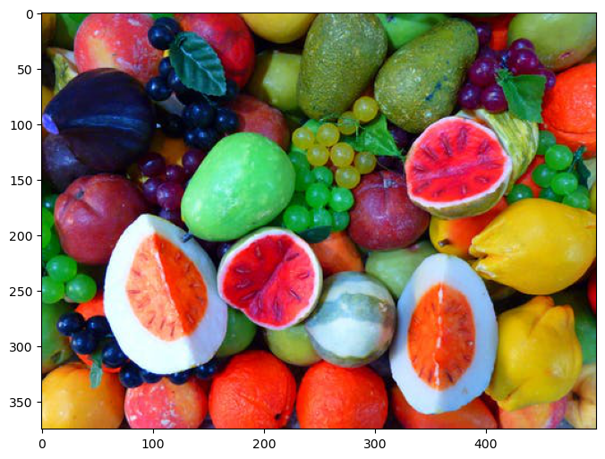
Load the fruits image.

# Load Data

mI = ski.io.imread(imgUrl)


print(f'The image shape: {mI.shape}')

The image shape: (375, 500, 3)

Plot Data

# Plot the Data

hF, hA = plt.subplots(figsize = (8, 8))

# Display the image
hA.imshow(mI)

plt.show()

Pre Processing

We need to convert the image from (numRows, numCols, numChannels) to (numRows * numCols, numChannels).
In our case, numChannels = 3 as we work with RGB image.

# Convert Image into Features Matrix

numRows, numCols, numChannel = mI.shape

#===========================Fill This===========================#
mX = np.reshape(mI, (numRows * numCols, numChannel))
#===============================================================#

print(f'The features data shape: {mX.shape}')

The features data shape: (187500, 3)

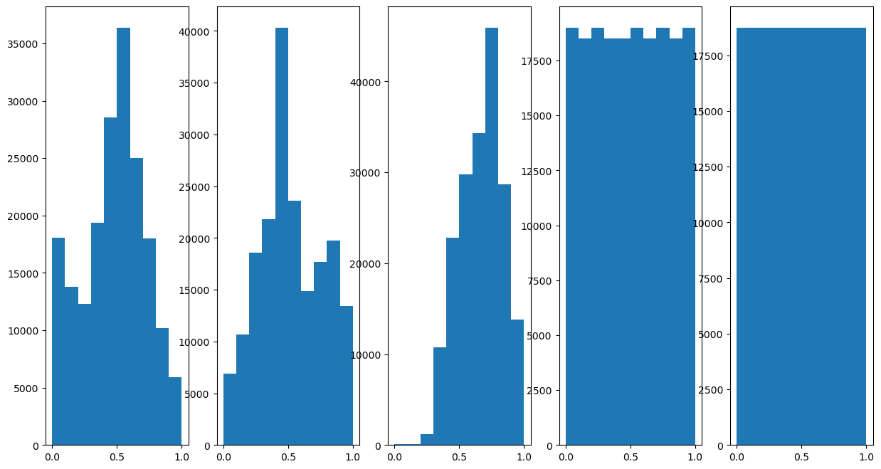
Feature Engineering

In this section we’ll apply the feature engineering:

1. Convert data into a meaningful color space (LAB).

2. Add the location (Row / Column indices) information as a feature to segment the image.

3. Scale features to have similar dynamic range.

# Convert Features into LAB Color Space
mX = ConvertRgbToLab(mX) #<! Have a look on the function

# Add the Indices as Features

#===========================Fill This===========================#
# 1. Create a vector of the row index of each pixel.
# 2. Create a vector of the column index of each pixel.
# 3. Stack them as additional columns to `mX`.
# !! Python is column major.
# !! The number of elements in the vectors should match the number of pixels.
# !! You may find `repeat()` and `tile()` functions (NumPy) useful.
vR = np.repeat(np.arange(numRows), repeats = numCols) #<! Row indices
vC = np.tile(np.arange(numCols), reps = numRows) #<! Column indices
mX = np.column_stack((mX, vR, vC))
#===============================================================#

numFeat = mX.shape[1]

print(f'The features data shape: {mX.shape}')

The features data shape: (187500, 5)

# Plot the Features Histogram 
hF, hA = plt.subplots(nrows = 1, ncols = numFeat, figsize = (15, 8))
hF = PlotFeaturesHist(mX, hF = hF)

# Scale Features
# Scale each feature into the [0, 1] range.
# Having similar scaling means have similar contribution when calculating the distance.

#===========================Fill This===========================#
# 1. Construct the `MinMaxScaler` object.
# 2. Use it to transform the data.
oMinMaxScaler = MinMaxScaler()
mX = oMinMaxScaler.fit_transform(mX)
#===============================================================#

• (?) What would happen if we didn’t scale the row and columns indices features?

# Plot the Features Histogram 
hF, hA = plt.subplots(nrows = 1, ncols = numFeat, figsize = (15, 8))
hF = PlotFeaturesHist(mX, hF = hF)

Cluster Data by K-Means

1. Step I:
   Assume fixed centroids \(\left\{ \boldsymbol{\mu}_{k}\right\} \), find the optimal clusters \(\left\{ \mathcal{D}_{k}\right\} \):
   $\(\arg\min_{\left\{ \mathcal{D}_{k}\right\} }\sum_{k = 1}^{K}\sum_{\boldsymbol{x}_{i}\in\mathcal{D}_{k}}\left\Vert \boldsymbol{x}_{i}-\boldsymbol{\mu}_{k}\right\Vert _{2}^{2}\)\( \)\(\implies \boldsymbol{x}_{i}\in\mathcal{D}_{s\left(\boldsymbol{x}_{i}\right)} \; \text{where} \; s\left(\boldsymbol{x}_{i}\right)=\arg\min_{k}\left\Vert \boldsymbol{x}_{i}-\boldsymbol{\mu}_{k}\right\Vert _{2}^{2}\)$

2. Step II:
   Assume fixed clusters \(\left\{ \mathcal{D}_{k}\right\} \), find the optimal centroids \(\left\{ \boldsymbol{\mu}_{k}\right\} \): $\(\arg\min_{\left\{ \boldsymbol{\mu}_{k}\right\} }\sum_{k=1}^{K}\sum_{\boldsymbol{x}_{i}\in\mathcal{D}_{k}}\left\Vert \boldsymbol{x}_{i}-\boldsymbol{\mu}_{k}\right\Vert _{2}^{2}\)\( \)\(\implies\boldsymbol{\mu}_{k}=\frac{1}{\left|\mathcal{D}_{k}\right|}\sum_{\boldsymbol{x}_{i}\in\mathcal{D}_{k}}\boldsymbol{x}_{i}\)$

3. Step III:
   Check for convergence (Change in assignments / location of the center). If not, go to Step I.

• (#) The K-Means is implemented in KMeans.

• (#) Some implementations of the algorithm supports different metrics.

• (?) With regard to the RGB features, is the metric used is the Squared Euclidean?

The K-Means Algorithm

Implement the K-Means algorithm as a SciKit Learn compatible class.

• (#) The implementation will allow different metrics.

# Implement the K-Means as an Estimator

class KMeansCluster(ClusterMixin, BaseEstimator):
    def __init__(self, numClusters: int, numIter: int = 1000, metricType: str = 'sqeuclidean'):
        #===========================Fill This===========================#
        # 1. Add `numClusters` as an attribute of the object.
        # 2. Add `numIter` as an attribute of the object.
        # 3. Add `metricType` as an attribute of the object.
        # !! The `metricType` must match the values of SciPy's `cdist()`: 'euclidean', 'cityblock', 'seuclidean', 'sqeuclidean', 'cosine', 'correlation'.
        self.numClusters = numClusters
        self.numIter     = numIter
        self.metricType  = metricType
        #===============================================================#

        pass
    
    def fit(self, mX: np.ndarray, vY: Optional[np.ndarray] = None) -> Self:

        numSamples  = mX.shape[0]
        featuresDim = mX.shape[1]

        if (numSamples < self.numClusters):
            raise ValueError(f'The number of samples: {numSamples} should not be smaller than the number of clusters: {self.numClusters}.')

        mC = mX[np.random.choice(numSamples, self.numClusters, replace = False)] #<! Centroids (Random initialization)
        vL = np.zeros(numSamples, dtype = np.int64) #<! Labels
        vF = np.zeros(numSamples, dtype = np.bool_) #<! Flags for each label
        
        #===========================Fill This===========================#
        # 1. Create a loop of the number of samples.
        # 2. Create the distance matrix between each sample to the centroids (Use the appropriate metrics).
        # 3. Extract the labels.
        # 4. Iterate on each label group to update the centroids.
        # !! You may find `cdist()` from SciPy useful.
        # !! Use `mean()` to calculate the centroids.
        for ii in range(self.numIter):
            mD = sp.spatial.distance.cdist(mX, mC, self.metricType) #<! Distance Matrix (numSamples, numClusters)
            vL = np.argmin(mD, axis = 1, out = vL)
            for kk in range(numClusters):
                # Update `mC`
                vF = np.equal(vL, kk, out = vF)
                if np.any(vF):
                    mC[kk, :] = np.mean(mX[vL == kk, :], axis = 0)
        #===============================================================#

        # SciKit Learn's `KMeans` compatibility
        self.cluster_centers_   = mC
        self.labels_            = vL
        self.inertia_           = np.sum(np.amin(mD, axis = 1))
        self.n_iter_            = self.numIter
        self.n_features_in      = featuresDim

        return self
    
    def transform(self, mX):

        return sp.spatial.distance.cdist(mX, self.cluster_centers_, self.metricType)
    
    def predict(self, mX):

        vL = np.argmin(self.transform(mX), axis = 1)

        return vL
    
    def score(self, mX: np.ndarray, vY: Optional[np.ndarray] = None):
        # Return the opposite of inertia as the score

        mD = self.transform(mX)
        inertiaVal = np.sum(np.amin(mD, axis = 1))

        return -inertiaVal

• (?) Why do the fit() and predict() method have the vY input?

• (?) If one selects 'cosine' as the distance metric, does the centroid match the metric?

• (@) Add an option for K-Means++ initialization.

• (?) How can one use K-Means in an online fashion? Think of a static and dynamic case.

• (?) Is the above implementation static or dynamic?

• (@) Add a stopping criteria: The maximum movement of a centroid is below a threshold.

Super Pixel Clustering by K-Means

# Construct the Model & Fit to Data

#===========================Fill This===========================#
# 1. Construct the `KMeansCluster` object.
# 2. Fit it to data.
oKMeans = KMeansCluster(numClusters = numClusters, numIter = numIter)
oKMeans = oKMeans.fit(mX)
#===============================================================#

• (?) What’s the difference between fit() and predict() in the context of K-Means?

# Extract the Labels and Form a Segmentation Mask

#===========================Fill This===========================#
# 1. Extract the labels of the pixels (Cluster index).
# 2. Reshape them into a mask which matches the image.
mSuperPixel = np.reshape(oKMeans.labels_, (numRows, numCols))
#===============================================================#

# Display Results

hF, hA = plt.subplots(figsize = (12, 8))
PlotSuperPixels(mI, mSuperPixel, hA = hA)

plt.show()

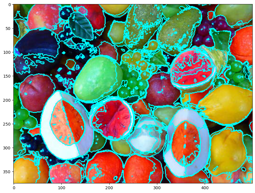
• (?) How do we set the hyper parameter K for K-Means?

• (?) Why are the separating lines not straight?

• (@) Run the notebook again yet using SciKit Learn KMeans class. Compare speed.

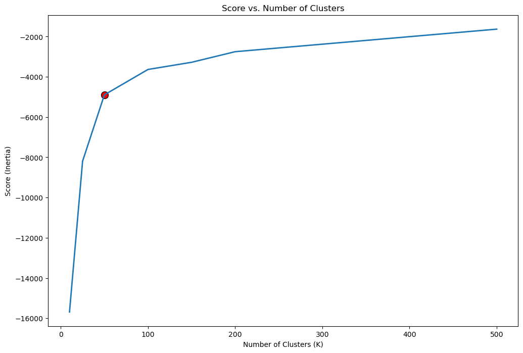
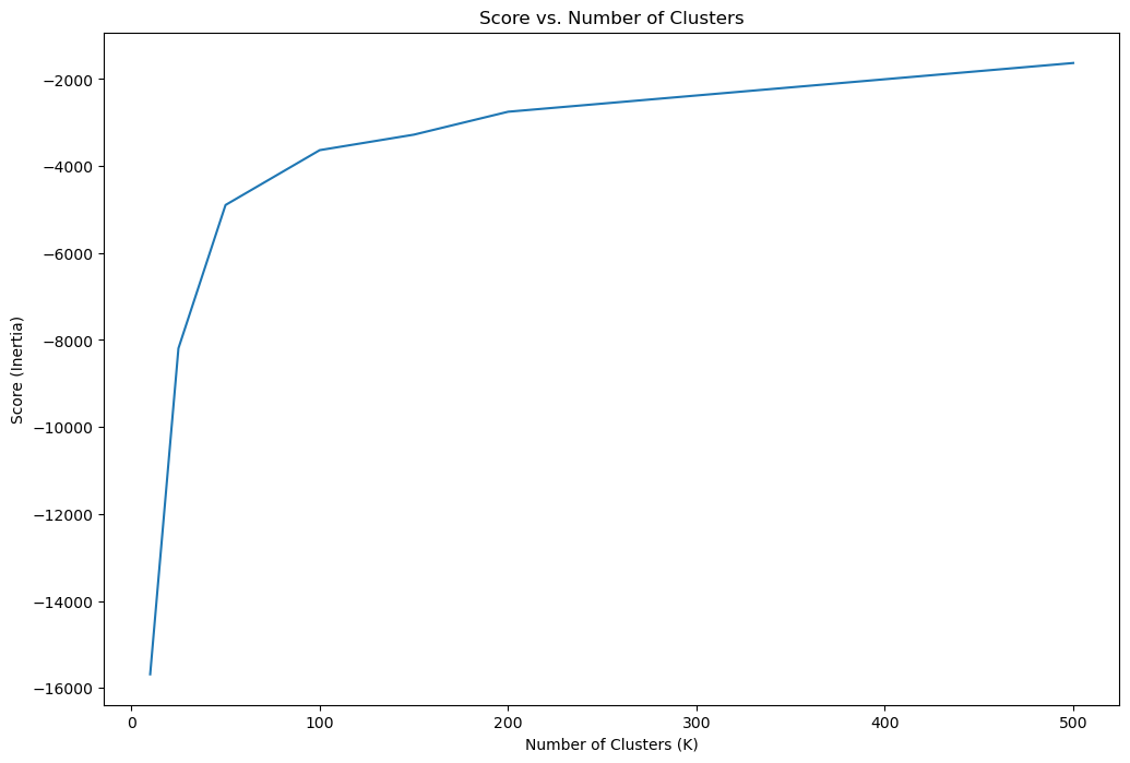
Analysis of Hyper Parameter K

One common method to find the optimal K is the Knee / Elbow Method.
In this method a score (Inertia) is plotted vs. the K parameter.
One way to define the elbow point is by the point maximizing the curvature.
This point can be easily calculated by the kneed package.

• (#) An alternative to the elbow method is using Silhouette. See Stop Using the Elbow Method, Selecting the Number of Clusters with Silhouette Analysis on KMeans Clustering.

• (#) Method to Analyze K in K-Means.

# Score per K
# Takes 4-6 minutes!
lK = [10, 25, 50, 100, 150, 200, 500]
numK = len(lK)
vS = np.full(shape = numK, fill_value = np.nan)

for ii, kVal in enumerate(lK):
    oKMeans = KMeansCluster(numClusters = kVal, numIter = numIter)
    oKMeans = oKMeans.fit(mX)
    vS[ii]  = oKMeans.score(mX)
    print(f'Finished processing the {ii} / {numK} iteration with K = {kVal}')

Finished processing the 0 / 7 iteration with K = 10
Finished processing the 1 / 7 iteration with K = 25
Finished processing the 2 / 7 iteration with K = 50
Finished processing the 3 / 7 iteration with K = 100
Finished processing the 4 / 7 iteration with K = 150
Finished processing the 5 / 7 iteration with K = 200
Finished processing the 6 / 7 iteration with K = 500

# Plot the Score
hF, hA = plt.subplots(figsize = (12, 8))
hA.plot(lK, vS, label = 'Score')
hA.set_xlabel('Number of Clusters (K)')
hA.set_ylabel('Score (Inertia)')
hA.set_title('Score vs. Number of Clusters')

plt.show()

# Locate the Knee Point by Maximum Curvature

oKneeLoc    = KneeLocator(lK, vS, curve = 'concave', direction = 'increasing')
kneeK       = round(oKneeLoc.knee)
kneeIdx     = lK.index(kneeK)

# Plot the Knee
hF, hA = plt.subplots(figsize = (12, 8))
hA.plot(lK, vS, lw = 2, label = 'Score')
hA.scatter(lK[kneeIdx], vS[kneeIdx], s = 100, c = 'r', edgecolors = 'k', label = 'Knee')
hA.set_xlabel('Number of Clusters (K)')
hA.set_ylabel('Score (Inertia)')
hA.set_title('Score vs. Number of Clusters')

plt.show()