Object Localization

Object Localization#

Notebook by:

Royi Avital RoyiAvital@fixelalgorithms.com

Revision History#

Version	Date	User	Content / Changes
1.0.000	08/06/2024	Royi Avital	First version

# Import Packages

# General Tools
import numpy as np
import scipy as sp
import pandas as pd

# Machine Learning
from sklearn.metrics import confusion_matrix, ConfusionMatrixDisplay
from sklearn.model_selection import ParameterGrid

# Deep Learning
import torch
import torch.nn            as nn
import torch.nn.functional as F
from torch.optim.optimizer import Optimizer
from torch.optim.lr_scheduler import LRScheduler
from torch.utils.data import DataLoader
from torch.utils.tensorboard import SummaryWriter
import torchinfo
from torchmetrics.classification import MulticlassAccuracy
from torchmetrics.detection.iou import IntersectionOverUnion

import torchvision
from torchvision.transforms import v2 as TorchVisionTrns

# Miscellaneous
import copy
from enum import auto, Enum, unique
import math
import os
from platform import python_version
import random
import shutil
import time

# Typing
from typing import Callable, Dict, Generator, List, Optional, Self, Set, Tuple, Union

# Visualization
import matplotlib as mpl
import matplotlib.pyplot as plt
import seaborn as sns

# Jupyter
from IPython import get_ipython
from IPython.display import HTML, Image
from IPython.display import display
from ipywidgets import Dropdown, FloatSlider, interact, IntSlider, Layout, SelectionSlider
from ipywidgets import interact

2024-06-15 04:40:45.389639: I tensorflow/core/platform/cpu_feature_guard.cc:182] This TensorFlow binary is optimized to use available CPU instructions in performance-critical operations.
To enable the following instructions: SSE4.1 SSE4.2 AVX AVX2 FMA, in other operations, rebuild TensorFlow with the appropriate compiler flags.

Notations#

(?) Question to answer interactively.
(!) Simple task to add code for the notebook.
(@) Optional / Extra self practice.
(#) Note / Useful resource / Food for thought.

Code Notations:

someVar    = 2; #<! Notation for a variable
vVector    = np.random.rand(4) #<! Notation for 1D array
mMatrix    = np.random.rand(4, 3) #<! Notation for 2D array
tTensor    = np.random.rand(4, 3, 2, 3) #<! Notation for nD array (Tensor)
tuTuple    = (1, 2, 3) #<! Notation for a tuple
lList      = [1, 2, 3] #<! Notation for a list
dDict      = {1: 3, 2: 2, 3: 1} #<! Notation for a dictionary
oObj       = MyClass() #<! Notation for an object
dfData     = pd.DataFrame() #<! Notation for a data frame
dsData     = pd.Series() #<! Notation for a series
hObj       = plt.Axes() #<! Notation for an object / handler / function handler

Code Exercise#

Single line fill

vallToFill = ???

Multi Line to Fill (At least one)

# You need to start writing
????

Section to Fill

#===========================Fill This===========================#
# 1. Explanation about what to do.
# !! Remarks to follow / take under consideration.
mX = ???

???
#===============================================================#

# Configuration
# %matplotlib inline

seedNum = 512
np.random.seed(seedNum)
random.seed(seedNum)

# Matplotlib default color palette
lMatPltLibclr = ['#1f77b4', '#ff7f0e', '#2ca02c', '#d62728', '#9467bd', '#8c564b', '#e377c2', '#7f7f7f', '#bcbd22', '#17becf']
# sns.set_theme() #>! Apply SeaBorn theme

runInGoogleColab = 'google.colab' in str(get_ipython())

# Improve performance by benchmarking
torch.backends.cudnn.benchmark = True

# Reproducibility (Per PyTorch Version on the same device)
# torch.manual_seed(seedNum)
# torch.backends.cudnn.deterministic = True
# torch.backends.cudnn.benchmark     = False #<! Makes things slower

# Constants

FIG_SIZE_DEF    = (8, 8)
ELM_SIZE_DEF    = 50
CLASS_COLOR     = ('b', 'r')
EDGE_COLOR      = 'k'
MARKER_SIZE_DEF = 10
LINE_WIDTH_DEF  = 2

DATA_SET_FILE_NAME      = 'archive.zip'
DATA_SET_FOLDER_NAME    = 'IntelImgCls'

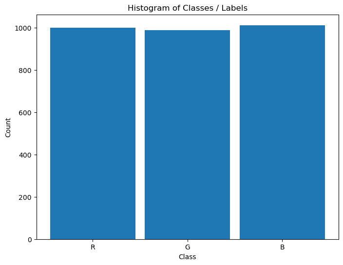
D_CLASSES  = {0: 'Red', 1: 'Green', 2: 'Blue'}
L_CLASSES  = ['R', 'G', 'B']
T_IMG_SIZE = (100, 100, 3)

DATA_FOLDER_PATH    = 'Data'
TENSOR_BOARD_BASE   = 'TB'

# Download Auxiliary Modules for Google Colab
if runInGoogleColab:
    !wget https://raw.githubusercontent.com/FixelAlgorithmsTeam/FixelCourses/master/AIProgram/2024_02/DataManipulation.py
    !wget https://raw.githubusercontent.com/FixelAlgorithmsTeam/FixelCourses/master/AIProgram/2024_02/DataVisualization.py
    !wget https://raw.githubusercontent.com/FixelAlgorithmsTeam/FixelCourses/master/AIProgram/2024_02/DeepLearningPyTorch.py

# Courses Packages
import sys
sys.path.append('../../utils')
sys.path.append('/home/vlad/utils')
from DataManipulation import BBoxFormat
from DataManipulation import GenLabeldEllipseImg
from DataVisualization import PlotBox, PlotBBox, PlotLabelsHistogram
from DeepLearningPyTorch import ObjectLocalizationDataset
from DeepLearningPyTorch import GenDataLoaders, InitWeightsKaiNorm, TrainModel, TrainModelSch

(!) Go through GenLabeldDataEllipse().
(!) Go through ObjectLocalizationDataset.

# General Auxiliary Functions

def GenResNetModel( trainedModel: bool, numCls: int, resNetDepth: int = 18 ) -> nn.Module:
    # Read on the API change at: How to Train State of the Art Models Using TorchVision’s Latest Primitives
    # https://pytorch.org/blog/how-to-train-state-of-the-art-models-using-torchvision-latest-primitives

    if (resNetDepth == 18):
        modelFun = torchvision.models.resnet18
        modelWeights = torchvision.models.ResNet18_Weights.IMAGENET1K_V1
    elif (resNetDepth == 34):
        modelFun = torchvision.models.resnet34
        modelWeights = torchvision.models.ResNet34_Weights.IMAGENET1K_V1
    else:
        raise ValueError(f'The `resNetDepth`: {resNetDepth} is invalid!')

    if trainedModel:
        oModel = modelFun(weights = modelWeights)
        numFeaturesIn   = oModel.fc.in_features
        # Assuming numCls << 100
        oModel.fc       = nn.Sequential(
            nn.Linear(numFeaturesIn, 128), nn.ReLU(),
            nn.Linear(128, numCls),
        )
    else:
        oModel = modelFun(weights = None, num_classes = numCls)

    return oModel


def GenData( numSamples: int, tuImgSize: Tuple[int, int, int], boxFormat: BBoxFormat = BBoxFormat.YOLO ) -> Tuple[np.ndarray, np.ndarray, np.ndarray]:

    mX = np.empty(shape = (numSamples, *tuImgSize[::-1]))
    vY = np.empty(shape = numSamples, dtype = np.int_)
    mB = np.empty(shape = (numSamples, 4))

    for ii in range(numSamples):
        mI, vLbl, mBB = GenLabeldEllipseImg(tuImgSize[:2], 1, boxFormat = boxFormat)
        mX[ii]  = np.transpose(mI, (2, 0, 1))
        vY[ii]  = vLbl[0]
        mB[ii]  = mBB[0]
    
    return mX, vY, mB
        
# Data Loader
# Using a function to mitigate Multi Process issues:
# https://pytorch.org/docs/stable/notes/windows.html#multiprocessing-error-without-if-clause-protection
def DataLoaderBatch( dlData: DataLoader ) -> Tuple:
    
    return next(iter(dlData)) #<! PyTorch Tensors

Object Localization#

The composability of Deep Learning loss allows combining 2 tasks into 1.
Object Localization is a composition of 2 tasks:

Classification: Identify the object class.
Regression: Localize the object by a Bounding Box (BB).

This notebook demonstrates:

Generating a synthetic data set.
Building a model for object localization
Training a model with a composed objective.

(#) In the notebook context Object Localization assumes the existence of an object in the image and only a single object.
(#) In the notebook context Object Detection generalizes the task to support the case of non existence or several objects.
(#) The motivation for a synthetic dataset is being able to implement the whole training process (Existing datasets are huge).
Yet the ability to create synthetic dataset is a useful skill.
(#) There are known datasets for object detection: COCO Dataset, PASCAL VOC.
They also define standards for the labeling system.
Training them is on the scale of days.
(#) Object Detection Annotation Formats.

# Parameters

# Data
numSamplesTrain = 30_000
numSamplesVal   = 10_000
boxFormat       = BBoxFormat.YOLO

# Model
dropP = 0.5 #<! Dropout Layer

# Training
batchSize   = 256
numWorkers  = 2 #<! Number of workers
numEpochs   = 35
λ = 20.0 #<! Localization Loss
ϵ = 0.1 #<! Label Smoothing

# Visualization
numImg = 3

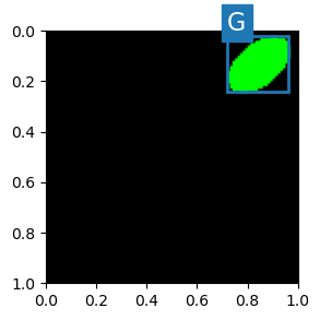
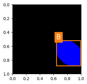
Generate / Load Data#

The data is synthetic data.
Each image includes and Ellipse where its color is the class (R, G, B) and the bounding rectangle.

(#) The label is a vector of 5: [Class, xCenter, yCenter, boxWidth, boxHeight].
(#) The label is in YOLO format, hence it is normalized to [0, 1].

# Image Sample

mI, vY, mBB = GenLabeldEllipseImg(T_IMG_SIZE[:2], 1, boxFormat = boxFormat)
vBox = mBB[0] #<! Matrix to support multiple objects in a single image
clsIdx = vY[0]
hA = PlotBox(mI, L_CLASSES[clsIdx], vBox)

../../../_images/8caea6038325db316e007d4119d7f70c53a306561d9c2b09b23a9eae0aa27fcc.png

(#) One could use negative values for the bounding box. The model will extrapolate the object dimensions.

## reduce to test
numSamplesTrain = 3_000
numSamplesVal   = 1_000

# Generate Data

mXTrain, vYTrain, mBBTrain = GenData(numSamplesTrain, T_IMG_SIZE, boxFormat = boxFormat)
mXVal,   vYVal,   mBBVal   = GenData(numSamplesVal, T_IMG_SIZE, boxFormat = boxFormat)

print(f'The training data set data shape: {mXTrain.shape}')
print(f'The training data set labels shape: {vYTrain.shape}')
print(f'The training data set box shape: {mBBTrain.shape}')
print(f'The validation data set data shape: {mXVal.shape}')
print(f'The validation data set labels shape: {vYTrain.shape}')
print(f'The validation data set box shape: {mBBVal.shape}')

The training data set data shape: (3000, 3, 100, 100)
The training data set labels shape: (3000,)
The training data set box shape: (3000, 4)
The validation data set data shape: (1000, 3, 100, 100)
The validation data set labels shape: (3000,)
The validation data set box shape: (1000, 4)

# Generate Data

dsTrain = ObjectLocalizationDataset(mXTrain, vYTrain, mBBTrain)
dsVal   = ObjectLocalizationDataset(mXVal, vYVal, mBBVal)
lClass  = list(dsTrain.vY)

print(f'The training data set data shape: {dsTrain.tX.shape}')
print(f'The test data set data shape: {dsVal.tX.shape}')
print(f'The unique values of the labels: {np.unique(lClass)}')

The training data set data shape: (3000, 3, 100, 100)
The test data set data shape: (1000, 3, 100, 100)
The unique values of the labels: [0 1 2]

(#) PyTorch with the v2 transforms deals with bounding boxes using special type: BoundingBoxes.
(#) For data augmentation see:

# Element of the Data Set

mX, vY = dsTrain[0]

valY    = int(vY[0])
vB      = vY[1:]

print(f'The features shape: {mX.shape}')
print(f'The label value: {valY}')
print(f'The bounding box value: {vB}')

The features shape: (3, 100, 100)
The label value: 0
The bounding box value: [0.175 0.8   0.35  0.36 ]

(#) Since the labels are in the same contiguous container as the bounding box parameters, their type is Float.
(#) The bounding box is using absolute values. In practice it is commonly normalized to the image dimensions.

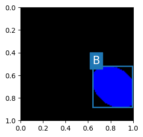
Plot the Data#

# Plot the Data

hA = PlotBox(np.transpose(mX, (1, 2, 0)), L_CLASSES[valY], vB)

../../../_images/03346f635b77cbfa5f5f3095ed73fadc3090db8bae31730a96cf3e848a79b603.png

# Histogram of Labels

hA = PlotLabelsHistogram(dsTrain.vY, lClass = L_CLASSES)
plt.show()

../../../_images/92e9e4fd7376db2ec23ebc9d3b3ad717b71c83adf138bc7cd2121eead3d3c452.png

Data Loaders#

This section defines the data loaded.

# Data Loader

dlTrain = torch.utils.data.DataLoader(dsTrain, shuffle = True, batch_size = 1 * batchSize, num_workers = numWorkers, drop_last = True, persistent_workers = True)
dlVal   = torch.utils.data.DataLoader(dsVal, shuffle = False, batch_size = 2 * batchSize, num_workers = numWorkers, persistent_workers = True)

# dlTrain = torch.utils.data.DataLoader(dsTrain, shuffle = True, batch_size = 1 * batchSize, num_workers = 0, drop_last = True, persistent_workers = False)
# dlVal   = torch.utils.data.DataLoader(dsVal, shuffle = False, batch_size = 2 * batchSize, num_workers = 0, persistent_workers = False)

# Iterate on the Loader
# The first batch.

tX, mY = DataLoaderBatch(dlTrain)

print(f'The batch features dimensions: {tX.shape}')
print(f'The batch labels dimensions: {mY[:, 0].shape}')
print(f'The batch bounding box dimensions: {mY[:, 1:].shape}')

The batch features dimensions: torch.Size([256, 3, 100, 100])
The batch labels dimensions: torch.Size([256])
The batch bounding box dimensions: torch.Size([256, 4])

The Model#

This section defines the model.

(#) The following implementation has a model with a single output, both for the regression and the classification.
(#) One could create 2 different outputs (Heads) for each task.

# Model
# Model generating function.

def BuildModel( numCls: int ) -> nn.Module:

    oModel = nn.Sequential(
        nn.Identity(),
        nn.Conv2d(3,   32,  3, stride = 2, padding = 0, bias = False), nn.BatchNorm2d(32 ), nn.ReLU(),
        nn.Conv2d(32,  32,  3, stride = 1, padding = 1, bias = False), nn.BatchNorm2d(32 ), nn.ReLU(),
        nn.Conv2d(32,  32,  3, stride = 2, padding = 0, bias = False), nn.BatchNorm2d(32 ), nn.ReLU(),
        nn.Conv2d(32,  32,  3, stride = 1, padding = 1, bias = False), nn.BatchNorm2d(32 ), nn.ReLU(),
        nn.Conv2d(32,  32,  3, stride = 1, padding = 1, bias = False), nn.BatchNorm2d(32 ), nn.ReLU(),
        nn.Conv2d(32,  64,  3, stride = 2, padding = 1, bias = False), nn.BatchNorm2d(64 ), nn.ReLU(),
        nn.Conv2d(64,  64,  3, stride = 1, padding = 1, bias = False), nn.BatchNorm2d(64 ), nn.ReLU(),
        nn.Conv2d(64,  64,  3, stride = 1, padding = 1, bias = False), nn.BatchNorm2d(64 ), nn.ReLU(),
        nn.Conv2d(64,  64,  3, stride = 1, padding = 1, bias = False), nn.BatchNorm2d(64 ), nn.ReLU(),
        nn.Conv2d(64,  64,  3, stride = 1, padding = 1, bias = False), nn.BatchNorm2d(64 ), nn.ReLU(),
        nn.Conv2d(64,  64,  3, stride = 2, padding = 1, bias = False), nn.BatchNorm2d(64 ), nn.ReLU(),
        nn.Conv2d(64,  128, 3, stride = 1, padding = 0, bias = False), nn.BatchNorm2d(128), nn.ReLU(),
        nn.Conv2d(128, 256, 3, stride = 1, padding = 0, bias = False), nn.BatchNorm2d(256), nn.ReLU(),
        nn.Conv2d(256, 512, 2, stride = 1, padding = 0, bias = False), nn.BatchNorm2d(512), nn.ReLU(),
        nn.Conv2d(512, numCls + 4, 1, stride = 1, padding = 0, bias = True),
        nn.Flatten()
    )

    return oModel 

notes#

(1) instead of fully connected at the end - we have a single output - with 1x1 pixel;

end of 1x1 pixel is like seeing in receptive field all the input image;

nn.Conv2d(512, numCls + 4, 1, stride = 1, padding = 0, bias = True),
nn.Flatten()

├─Conv2d (43): 1-44                      [1, 1]                    [256, 7, 1, 1]            3,591

    convulsion 1*1 - 7 times

├─Flatten (44): 1-45                     --                        [256, 7]                  --

****   it the same like linear FC =>  512 * 7 + 7  = 3591

(2) why so deep and so many layers?

for RF to include all the ellipse ; each pixel at the end must know if he inside the ellipse
calc RF ?

(3) used input of 100x100 can do the same for other size input?

input of 20x20 cant - less then 100x100 cant go to 1x1…
120x120 can work but wont finish with 1x1 - so need to resize and crop to 100x100

# Build the Model

oModel = BuildModel(len(L_CLASSES))

# Model Information - Pre Defined
# Pay attention to the layers name.
torchinfo.summary(oModel, (batchSize, *(T_IMG_SIZE[::-1])), col_names = ['kernel_size', 'output_size', 'num_params'], device = 'cpu', row_settings = ['depth', 'var_names'])

===================================================================================================================
Layer (type (var_name):depth-idx)        Kernel Shape              Output Shape              Param #
===================================================================================================================
Sequential (Sequential)                  --                        [256, 7]                  --
├─Identity (0): 1-1                      --                        [256, 3, 100, 100]        --
├─Conv2d (1): 1-2                        [3, 3]                    [256, 32, 49, 49]         864
├─BatchNorm2d (2): 1-3                   --                        [256, 32, 49, 49]         64
├─ReLU (3): 1-4                          --                        [256, 32, 49, 49]         --
├─Conv2d (4): 1-5                        [3, 3]                    [256, 32, 49, 49]         9,216
├─BatchNorm2d (5): 1-6                   --                        [256, 32, 49, 49]         64
├─ReLU (6): 1-7                          --                        [256, 32, 49, 49]         --
├─Conv2d (7): 1-8                        [3, 3]                    [256, 32, 24, 24]         9,216
├─BatchNorm2d (8): 1-9                   --                        [256, 32, 24, 24]         64
├─ReLU (9): 1-10                         --                        [256, 32, 24, 24]         --
├─Conv2d (10): 1-11                      [3, 3]                    [256, 32, 24, 24]         9,216
├─BatchNorm2d (11): 1-12                 --                        [256, 32, 24, 24]         64
├─ReLU (12): 1-13                        --                        [256, 32, 24, 24]         --
├─Conv2d (13): 1-14                      [3, 3]                    [256, 32, 24, 24]         9,216
├─BatchNorm2d (14): 1-15                 --                        [256, 32, 24, 24]         64
├─ReLU (15): 1-16                        --                        [256, 32, 24, 24]         --
├─Conv2d (16): 1-17                      [3, 3]                    [256, 64, 12, 12]         18,432
├─BatchNorm2d (17): 1-18                 --                        [256, 64, 12, 12]         128
├─ReLU (18): 1-19                        --                        [256, 64, 12, 12]         --
├─Conv2d (19): 1-20                      [3, 3]                    [256, 64, 12, 12]         36,864
├─BatchNorm2d (20): 1-21                 --                        [256, 64, 12, 12]         128
├─ReLU (21): 1-22                        --                        [256, 64, 12, 12]         --
├─Conv2d (22): 1-23                      [3, 3]                    [256, 64, 12, 12]         36,864
├─BatchNorm2d (23): 1-24                 --                        [256, 64, 12, 12]         128
├─ReLU (24): 1-25                        --                        [256, 64, 12, 12]         --
├─Conv2d (25): 1-26                      [3, 3]                    [256, 64, 12, 12]         36,864
├─BatchNorm2d (26): 1-27                 --                        [256, 64, 12, 12]         128
├─ReLU (27): 1-28                        --                        [256, 64, 12, 12]         --
├─Conv2d (28): 1-29                      [3, 3]                    [256, 64, 12, 12]         36,864
├─BatchNorm2d (29): 1-30                 --                        [256, 64, 12, 12]         128
├─ReLU (30): 1-31                        --                        [256, 64, 12, 12]         --
├─Conv2d (31): 1-32                      [3, 3]                    [256, 64, 6, 6]           36,864
├─BatchNorm2d (32): 1-33                 --                        [256, 64, 6, 6]           128
├─ReLU (33): 1-34                        --                        [256, 64, 6, 6]           --
├─Conv2d (34): 1-35                      [3, 3]                    [256, 128, 4, 4]          73,728
├─BatchNorm2d (35): 1-36                 --                        [256, 128, 4, 4]          256
├─ReLU (36): 1-37                        --                        [256, 128, 4, 4]          --
├─Conv2d (37): 1-38                      [3, 3]                    [256, 256, 2, 2]          294,912
├─BatchNorm2d (38): 1-39                 --                        [256, 256, 2, 2]          512
├─ReLU (39): 1-40                        --                        [256, 256, 2, 2]          --
├─Conv2d (40): 1-41                      [2, 2]                    [256, 512, 1, 1]          524,288
├─BatchNorm2d (41): 1-42                 --                        [256, 512, 1, 1]          1,024
├─ReLU (42): 1-43                        --                        [256, 512, 1, 1]          --
├─Conv2d (43): 1-44                      [1, 1]                    [256, 7, 1, 1]            3,591
├─Flatten (44): 1-45                     --                        [256, 7]                  --
===================================================================================================================
Total params: 1,139,879
Trainable params: 1,139,879
Non-trainable params: 0
Total mult-adds (Units.GIGABYTES): 17.47
===================================================================================================================
Input size (MB): 30.72
Forward/backward pass size (MB): 1068.78
Params size (MB): 4.56
Estimated Total Size (MB): 1104.06
===================================================================================================================

(?) Explain the dimensions of the last layer.
(?) Will the model work with smaller images?

Train the Model#

This section trains the model.

(#) The training loop must be adapted to the new loss function.

Image Localization Loss#

The loss is a composite of 2 loss functions:

\[\ell\left(\hat{\boldsymbol{y}},\boldsymbol{y}\right)=\lambda_{\text{MSE}}\cdot\ell_{\text{MSE}}\left(\hat{\boldsymbol{y}}_{\text{bbox}},\boldsymbol{y}_{\text{bbox}}\right)+\lambda_{\text{CE}}\cdot\ell_{\text{CE}}\left(\hat{\boldsymbol{y}}_{\text{label}},\boldsymbol{y}_{\text{label}}\right)\]

Where \(\lambda_{\text{MSE}}\) and \(\lambda_{\text{CE}}\) are the weights of each loss.

(#) In practice a single \(\lambda\) is required.
(#) The MSE is not optimal loss function. It will be replaced by the Log Euclidean loss.

# Object Localization Loss
class ObjLocLoss( nn.Module ):
    def __init__( self, numCls: int, λ: float, ϵ: float = 0.0 ) -> None:
        super(ObjLocLoss, self).__init__()

        self.numCls     = numCls
        self.λ          = λ
        self.ϵ          = ϵ
        self.oMseLoss   = nn.MSELoss()
        self.oCeLoss    = nn.CrossEntropyLoss(label_smoothing = ϵ)
    
    def forward( self: Self, mYHat: torch.Tensor, mY: torch.Tensor ) -> torch.Tensor:

        mseLoss = self.oMseLoss(mYHat[:, self.numCls:], mY[:, 1:])
        ceLoss  = self.oCeLoss(mYHat[:, :self.numCls], mY[:, 0].to(torch.long))

        lossVal = (self.λ * mseLoss) + ceLoss
		
        return lossVal

Image Localization Score#

The score is defined by the IoU of a valid classification:

\[\text{Metric}=\frac{1}{N}\sum_{i=1}^{N}\mathbb{I}\left\{ \hat{y}_{i}=y_{i}\right\} \cdot\text{IoU}\left(\hat{B}_{i},B_{i}\right)\]

Where:

\(\hat{y}_{i}\) is the predicted label
\(y_{i}\) is the correct label
\(\hat{B}_{i}\) is the predicted bounding box
\(B_{i}\) is the correct bounding box In other words, the average IoU, considering only correct (label) prediction.

# Object Localization Score
class ObjLocScore( nn.Module ):
    def __init__( self, numCls: int ) -> None:
        super(ObjLocScore, self).__init__()

        self.numCls = numCls
    
    def forward( self: Self, mYHat: torch.Tensor, mY: torch.Tensor ) -> Tuple[float, float, float]:

        batchSize = mYHat.shape[0]
        
        vY, mBox = mY[:, 0].to(torch.long), mY[:, 1:]

        vIoU = torch.diag(torchvision.ops.box_iou(torchvision.ops.box_convert(mYHat[:, self.numCls:], 'cxcywh', 'xyxy'), torchvision.ops.box_convert(mBox, 'cxcywh', 'xyxy')))
        vCor = (vY == torch.argmax(mYHat[:, :self.numCls], dim = 1)).to(torch.float32) #<! Correct labels

        # valIoU      = torch.mean(vIoU).item()
        # valAcc      = torch.mean(vCor).item()
        valScore    = torch.inner(vIoU, vCor) / batchSize
		
        return valScore

# Run Device

runDevice = torch.device('cuda:0' if torch.cuda.is_available() else 'cpu') #<! The 1st CUDA device

# Loss and Score Function

hL = ObjLocLoss(numCls = len(L_CLASSES), λ = λ, ϵ = ϵ)
hS = ObjLocScore(numCls = len(L_CLASSES))

hL = hL.to(runDevice)
hS = hS.to(runDevice)

# Training Loop

oModel = oModel.to(runDevice)
oOpt = torch.optim.AdamW(oModel.parameters(), lr = 1e-5, betas = (0.9, 0.99), weight_decay = 1e-5) #<! Define optimizer
oSch = torch.optim.lr_scheduler.OneCycleLR(oOpt, max_lr = 5e-4, total_steps = numEpochs)
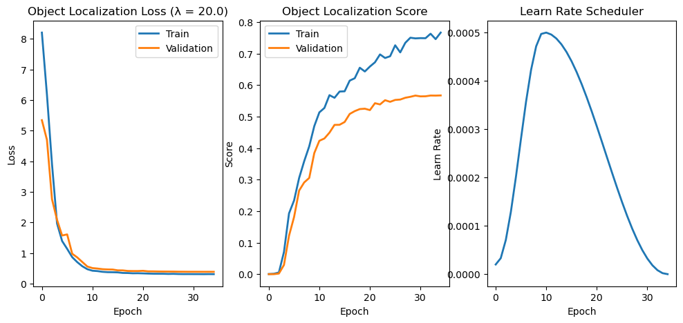
_, lTrainLoss, lTrainScore, lValLoss, lValScore, lLearnRate = TrainModel(oModel, dlTrain, dlVal, oOpt, numEpochs, hL, hS, oSch = oSch)

Epoch    1 / 35 | Train Loss:  8.204 | Val Loss:  5.342 | Train Score:  0.000 | Val Score:  0.000 | Epoch Time: 14.86 | <-- Checkpoint! |
Epoch    2 / 35 | Train Loss:  6.180 | Val Loss:  4.699 | Train Score:  0.001 | Val Score:  0.000 | Epoch Time:  1.26 |
Epoch    3 / 35 | Train Loss:  3.907 | Val Loss:  2.758 | Train Score:  0.005 | Val Score:  0.002 | Epoch Time:  1.23 | <-- Checkpoint! |
Epoch    4 / 35 | Train Loss:  1.965 | Val Loss:  2.085 | Train Score:  0.070 | Val Score:  0.029 | Epoch Time:  1.23 | <-- Checkpoint! |
Epoch    5 / 35 | Train Loss:  1.393 | Val Loss:  1.573 | Train Score:  0.193 | Val Score:  0.122 | Epoch Time:  1.23 | <-- Checkpoint! |
Epoch    6 / 35 | Train Loss:  1.136 | Val Loss:  1.609 | Train Score:  0.234 | Val Score:  0.181 | Epoch Time:  1.24 | <-- Checkpoint! |
Epoch    7 / 35 | Train Loss:  0.865 | Val Loss:  0.976 | Train Score:  0.305 | Val Score:  0.265 | Epoch Time:  1.23 | <-- Checkpoint! |
Epoch    8 / 35 | Train Loss:  0.702 | Val Loss:  0.856 | Train Score:  0.358 | Val Score:  0.291 | Epoch Time:  1.23 | <-- Checkpoint! |
Epoch    9 / 35 | Train Loss:  0.568 | Val Loss:  0.706 | Train Score:  0.406 | Val Score:  0.305 | Epoch Time:  1.23 | <-- Checkpoint! |
Epoch   10 / 35 | Train Loss:  0.471 | Val Loss:  0.558 | Train Score:  0.470 | Val Score:  0.384 | Epoch Time:  1.24 | <-- Checkpoint! |
Epoch   11 / 35 | Train Loss:  0.422 | Val Loss:  0.508 | Train Score:  0.513 | Val Score:  0.423 | Epoch Time:  1.23 | <-- Checkpoint! |
Epoch   12 / 35 | Train Loss:  0.410 | Val Loss:  0.493 | Train Score:  0.527 | Val Score:  0.430 | Epoch Time:  1.24 | <-- Checkpoint! |
Epoch   13 / 35 | Train Loss:  0.386 | Val Loss:  0.472 | Train Score:  0.568 | Val Score:  0.449 | Epoch Time:  1.23 | <-- Checkpoint! |
Epoch   14 / 35 | Train Loss:  0.375 | Val Loss:  0.463 | Train Score:  0.560 | Val Score:  0.474 | Epoch Time:  1.24 | <-- Checkpoint! |
Epoch   15 / 35 | Train Loss:  0.373 | Val Loss:  0.460 | Train Score:  0.579 | Val Score:  0.474 | Epoch Time:  1.23 | <-- Checkpoint! |
Epoch   16 / 35 | Train Loss:  0.367 | Val Loss:  0.434 | Train Score:  0.580 | Val Score:  0.483 | Epoch Time:  1.23 | <-- Checkpoint! |
Epoch   17 / 35 | Train Loss:  0.349 | Val Loss:  0.433 | Train Score:  0.614 | Val Score:  0.508 | Epoch Time:  1.24 | <-- Checkpoint! |
Epoch   18 / 35 | Train Loss:  0.346 | Val Loss:  0.414 | Train Score:  0.622 | Val Score:  0.517 | Epoch Time:  1.23 | <-- Checkpoint! |
Epoch   19 / 35 | Train Loss:  0.338 | Val Loss:  0.412 | Train Score:  0.655 | Val Score:  0.524 | Epoch Time:  1.23 | <-- Checkpoint! |
Epoch   20 / 35 | Train Loss:  0.340 | Val Loss:  0.412 | Train Score:  0.643 | Val Score:  0.525 | Epoch Time:  1.23 | <-- Checkpoint! |
Epoch   21 / 35 | Train Loss:  0.335 | Val Loss:  0.419 | Train Score:  0.659 | Val Score:  0.521 | Epoch Time:  1.23 |
Epoch   22 / 35 | Train Loss:  0.329 | Val Loss:  0.402 | Train Score:  0.672 | Val Score:  0.542 | Epoch Time:  1.23 | <-- Checkpoint! |
Epoch   23 / 35 | Train Loss:  0.324 | Val Loss:  0.401 | Train Score:  0.697 | Val Score:  0.539 | Epoch Time:  1.24 |
Epoch   24 / 35 | Train Loss:  0.323 | Val Loss:  0.397 | Train Score:  0.686 | Val Score:  0.552 | Epoch Time:  1.23 | <-- Checkpoint! |
Epoch   25 / 35 | Train Loss:  0.322 | Val Loss:  0.395 | Train Score:  0.691 | Val Score:  0.547 | Epoch Time:  1.24 |
Epoch   26 / 35 | Train Loss:  0.317 | Val Loss:  0.394 | Train Score:  0.726 | Val Score:  0.553 | Epoch Time:  1.23 | <-- Checkpoint! |
Epoch   27 / 35 | Train Loss:  0.320 | Val Loss:  0.393 | Train Score:  0.704 | Val Score:  0.554 | Epoch Time:  1.23 | <-- Checkpoint! |
Epoch   28 / 35 | Train Loss:  0.314 | Val Loss:  0.390 | Train Score:  0.734 | Val Score:  0.560 | Epoch Time:  1.24 | <-- Checkpoint! |
Epoch   29 / 35 | Train Loss:  0.312 | Val Loss:  0.389 | Train Score:  0.750 | Val Score:  0.563 | Epoch Time:  1.23 | <-- Checkpoint! |
Epoch   30 / 35 | Train Loss:  0.312 | Val Loss:  0.388 | Train Score:  0.748 | Val Score:  0.567 | Epoch Time:  1.23 | <-- Checkpoint! |
Epoch   31 / 35 | Train Loss:  0.311 | Val Loss:  0.388 | Train Score:  0.749 | Val Score:  0.564 | Epoch Time:  1.24 |
Epoch   32 / 35 | Train Loss:  0.311 | Val Loss:  0.387 | Train Score:  0.749 | Val Score:  0.564 | Epoch Time:  1.27 |
Epoch   33 / 35 | Train Loss:  0.310 | Val Loss:  0.387 | Train Score:  0.763 | Val Score:  0.567 | Epoch Time:  1.28 | <-- Checkpoint! |
Epoch   34 / 35 | Train Loss:  0.312 | Val Loss:  0.387 | Train Score:  0.746 | Val Score:  0.567 | Epoch Time:  1.25 |
Epoch   35 / 35 | Train Loss:  0.310 | Val Loss:  0.387 | Train Score:  0.766 | Val Score:  0.567 | Epoch Time:  1.26 | <-- Checkpoint! |

# Plot Training Phase

hF, vHa = plt.subplots(nrows = 1, ncols = 3, figsize = (12, 5))
vHa = np.ravel(vHa)

hA = vHa[0]
hA.plot(lTrainLoss, lw = 2, label = 'Train')
hA.plot(lValLoss, lw = 2, label = 'Validation')
hA.set_title(f'Object Localization Loss (λ = {λ:0.1f})')
hA.set_xlabel('Epoch')
hA.set_ylabel('Loss')
hA.legend()

hA = vHa[1]
hA.plot(lTrainScore, lw = 2, label = 'Train')
hA.plot(lValScore, lw = 2, label = 'Validation')
hA.set_title('Object Localization Score')
hA.set_xlabel('Epoch')
hA.set_ylabel('Score')
hA.legend()

hA = vHa[2]
hA.plot(lLearnRate, lw = 2)
hA.set_title('Learn Rate Scheduler')
hA.set_xlabel('Epoch')
hA.set_ylabel('Learn Rate')

Text(0, 0.5, 'Learn Rate')

../../../_images/c530fa0c3d28e0666e575b68eec748009fed694bd699d9d5ae9777ba6be94438.png

# Plot Prediction

rndIdx = np.random.randint(numSamplesVal)

mX, vY = dsVal[rndIdx]
valY    = int(vY[0])
vB      = vY[1:]
with torch.no_grad():
    tX = torch.tensor(mX)
    tX = torch.unsqueeze(tX, 0)
    tX = tX.to(runDevice)
    mYHat = oModel(tX).detach().cpu().numpy()

vYHat       = mYHat[0]
valYHat     = int(vYHat[0])
vBHat       = vY[1:]

hA = PlotBox(np.transpose(mX, (1, 2, 0)), L_CLASSES[valY], vB)
hA = PlotBBox(hA, L_CLASSES[valYHat], vBHat)

../../../_images/2aff1b2c40a475714552fb1b8f53d32cddb1440a5afa7b89bbadbd15d9c982a5.png

(@) Display the accuracy and IoU scores and MSE and CE loss over the epochs.
It will require updating the Loss, Score classes and the training function.

Object Localization

Contents

Object Localization#

Revision History#

Notations#

Code Exercise#

Object Localization#

Generate / Load Data#

Plot the Data#

Data Loaders#

The Model#

notes#

Train the Model#

Image Localization Loss#

Image Localization Score#