
Polynomial Fit with RANSAC#
Notebook by:
Royi Avital RoyiAvital@fixelalgorithms.com
Revision History#
Version |
Date |
User |
Content / Changes |
|---|---|---|---|
1.0.000 |
24/03/2024 |
Royi Avital |
First version |
![]()
# Import Packages

# General Tools
import numpy as np
import scipy as sp
import pandas as pd

# Machine Learning
from sklearn.linear_model import HuberRegressor, LinearRegression ,RANSACRegressor

# Miscellaneous
import math
import os
from platform import python_version
import random
import timeit

# Typing
from typing import Callable, Dict, List, Optional, Set, Tuple, Union

# Visualization
import matplotlib as mpl
import matplotlib.pyplot as plt
import seaborn as sns

# Jupyter
from IPython import get_ipython
from IPython.display import Image
from IPython.display import display
from ipywidgets import Dropdown, FloatSlider, interact, IntSlider, Layout, SelectionSlider
from ipywidgets import interact
Notations#
(?) Question to answer interactively.
(!) Simple task to add code for the notebook.
(@) Optional / Extra self practice.
(#) Note / Useful resource / Food for thought.
Code Notations:
someVar    = 2; #<! Notation for a variable
vVector    = np.random.rand(4) #<! Notation for 1D array
mMatrix    = np.random.rand(4, 3) #<! Notation for 2D array
tTensor    = np.random.rand(4, 3, 2, 3) #<! Notation for nD array (Tensor)
tuTuple    = (1, 2, 3) #<! Notation for a tuple
lList      = [1, 2, 3] #<! Notation for a list
dDict      = {1: 3, 2: 2, 3: 1} #<! Notation for a dictionary
oObj       = MyClass() #<! Notation for an object
dfData     = pd.DataFrame() #<! Notation for a data frame
dsData     = pd.Series() #<! Notation for a series
hObj       = plt.Axes() #<! Notation for an object / handler / function handler
Code Exercise#
Single line fill
vallToFill = ???
Multi Line to Fill (At least one)
# You need to start writing
????
Section to Fill
#===========================Fill This===========================#
# 1. Explanation about what to do.
# !! Remarks to follow / take under consideration.
mX = ???

???
#===============================================================#
# Configuration
# %matplotlib inline

seedNum = 512
np.random.seed(seedNum)
random.seed(seedNum)

# Matplotlib default color palette
lMatPltLibclr = ['#1f77b4', '#ff7f0e', '#2ca02c', '#d62728', '#9467bd', '#8c564b', '#e377c2', '#7f7f7f', '#bcbd22', '#17becf']
# sns.set_theme() #>! Apply SeaBorn theme

runInGoogleColab = 'google.colab' in str(get_ipython())
# Constants

FIG_SIZE_DEF    = (8, 8)
ELM_SIZE_DEF    = 50
CLASS_COLOR     = ('b', 'r')
EDGE_COLOR      = 'k'
MARKER_SIZE_DEF = 10
LINE_WIDTH_DEF  = 2
# Courses Packages

import sys
sys.path.append('../')
sys.path.append('../../')
sys.path.append('../../../')
from utils.DataVisualization import PlotRegressionData
# General Auxiliary Functions

def GenOutlierData( vR: np.ndarray, vO: np.ndarray, vI: np.ndarray, numOutliers: int ) -> np.ndarray:

    vY = vR.copy()
    vY[vI[:numOutliers]] = vO[vI[:numOutliers]]

    return vY

def PlotPolyFit( vX: np.ndarray, vR: np.ndarray, vO: np.ndarray, vI: np.ndarray, numOutliers: int, P: int, minSamplesRatio: float,
                numGridPts: int = 1001, hA: Optional[plt.Axes] = None, figSize: Tuple[int, int] = FIG_SIZE_DEF, markerSize: int = MARKER_SIZE_DEF,
                lineWidth: int = LINE_WIDTH_DEF, axisTitle: Optional[str] = None ) -> None:

    if hA is None:
        hF, hA = plt.subplots(1, 1, figsize = figSize)
    else:
        hF = hA[0].get_figure()

    numSamples = len(vX)

    mX = vX[:, np.newaxis] ** range(P + 1)
    vY = GenOutlierData(vR, vO, vI, numOutliers)

    oLinReg = LinearRegression(fit_intercept = False).fit(mX, vY)
    oRanReg = RANSACRegressor(estimator = LinearRegression(fit_intercept = False), min_samples = minSamplesRatio).fit(mX, vY)
    oHubReg = HuberRegressor(fit_intercept = False).fit(mX, vY)

    #TODO: Add calculation of the R2 only on the inliers

    # Plot
    xx  = np.linspace(np.floor(np.min(vX)), np.ceil(np.max(vX)), numGridPts)
    yy1 = np.polyval(oLinReg.coef_[::-1], xx)
    yy2 = np.polyval(oRanReg.estimator_.coef_[::-1], xx)
    yy3 = np.polyval(oHubReg.coef_[::-1], xx)

    hA.plot(vX, vY, '.r', ms = markerSize, label = '$y_i$')
    hA.plot(vX[vI[:numOutliers]], vY[vI[:numOutliers]], '.y', ms = markerSize, label = 'Outliers')
    hA.plot(xx, yy1, 'g', lw = 2,  label = f'OLS, R2 = {oLinReg.score(mX, vY)}')
    hA.plot(xx, yy2, 'b', lw = 2,  label = f'RANSAC, R2 = {oRanReg.estimator_.score(mX, vY)}')
    hA.plot(xx, yy3, 'm', lw = 2,  label = f'Huber, R2 = {oHubReg.score(mX, vY)}')
    hA.set_title (f'OLS vs. RANSAC OLS vs. Huber Loss')
    hA.set_xlabel('$x$')
    hA.set_ylabel('$y$')
    hA.grid()
    hA.legend()
Robust Regression#
The concept of Robust Regression is to estimate the model parameters while minimizing the effect of the outliers.
It is usually achieved by 2 approaches:
Robust Objective
Using an outlier robust objective function. Such as the \({L}^{1}\) or Huber Loss.Filtration
Marking the outliers and applying the objective on the inliers.
(#) RANSAC is a filtration approach which iteratively finds the inliers of the data.
# Parameters

# Data Generation
numSamples  = 150
noiseStd    = 0.3
numOutliers = 30
fctOutliers = 5

vP = np.array([1, 2])

# Data Visualization
gridNoiseStd    = 0.05
numGridPts      = 500
Generate / Load Data#
Where
# The Data Generating Function

def f( vX: np.ndarray, vP: np.ndarray ) -> np.ndarray:

    return np.polyval(vP, vX)

hF = lambda vX: f(vX, vP)
# Generate Data

vX = np.linspace(-2, 2, numSamples, endpoint = True) + (gridNoiseStd * np.random.randn(numSamples))
vN = noiseStd * np.random.randn(numSamples)
vR = f(vX, vP) + vN
vO = fctOutliers * vR
vI = np.random.permutation(numSamples)
vY = GenOutlierData(vR, vO, vI, numOutliers)

print(f'The features data shape: {vX.shape}')
print(f'The labels data shape: {vY.shape}')
The features data shape: (150,)
The labels data shape: (150,)
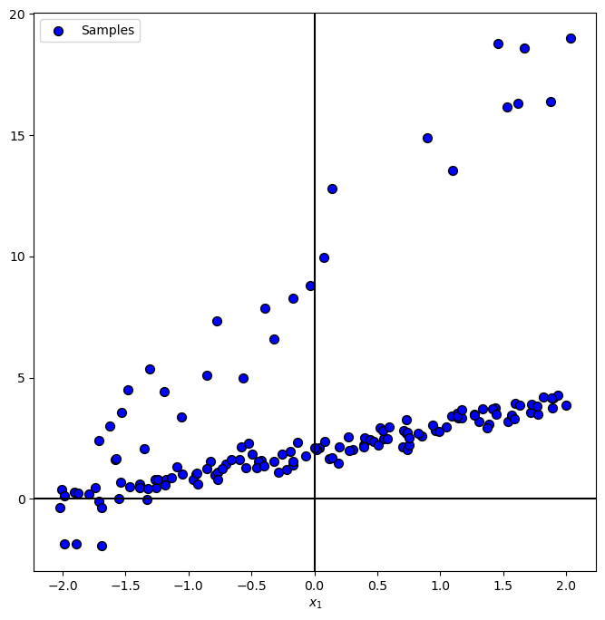
Plot Data#
# Plot the Data

PlotRegressionData(vX, vY)

plt.show()
Train a Robust Polyfit Regressor#
The Linear Regressor optimization problem is given by:
Where in Polynomial model:
There are 2 robust model to train:
Huber Loss
Being based on a Robust Loss.
Implemented byHuberRegressor.RANSAC Filtration of outliers by maximizing the number of inliers. Implemented by
RANSACRegressor.
The modelestimatorparameter supports any regressor with thefit(),predict()andscore()methods.
(#) Linear model can work with any features with transformation (Polynomial or not).
(#) In practice the RANSAC method can be used for any model, Linear or Non Linear.
# Interactive Plot

hPolyFit = lambda numOutliers, minSamplesRatio: PlotPolyFit(vX, vR, vO, vI, numOutliers, len(vP) - 1, minSamplesRatio)
numOutliersSlider = IntSlider(min = 0, max = numSamples, step = 1, value = 0, layout = Layout(width = '30%'))
minSamplesRatioSlider = FloatSlider(min = 0.01, max = 1.0, step = 0.01, value = 0.5, layout = Layout(width = '30%'))
interact(hPolyFit, numOutliers = numOutliersSlider, minSamplesRatio = minSamplesRatioSlider)
plt.show()
(?) Does the R2 score reflects the performance? What can be done?
(#) Once we have the model we may even use it to identify the outliers (Outlier / Anomaly Detection).
R2 score examples:
