
Label Smoothing#
Notebook by:
Royi Avital RoyiAvital@fixelalgorithms.com
Revision History#
Version |
Date |
User |
Content / Changes |
|---|---|---|---|
1.0.000 |
04/06/2024 |
Royi Avital |
First version |
![]()
# Import Packages

# General Tools
import numpy as np
import scipy as sp
import pandas as pd

# Machine Learning
from sklearn.metrics import confusion_matrix, ConfusionMatrixDisplay
from sklearn.model_selection import ParameterGrid

# Deep Learning
import torch
import torch.nn            as nn
import torch.nn.functional as F
from torch.optim.optimizer import Optimizer
from torch.optim.lr_scheduler import LRScheduler
from torch.utils.data import DataLoader
from torch.utils.tensorboard import SummaryWriter
import torchinfo
from torchmetrics.classification import MulticlassAccuracy
import torchvision
from torchvision.transforms import v2 as TorchVisionTrns

# Miscellaneous
import copy
from enum import auto, Enum, unique
import math
import os
from platform import python_version
import random
import shutil
import time

# Typing
from typing import Callable, Dict, Generator, List, Optional, Self, Set, Tuple, Union

# Visualization
import matplotlib as mpl
import matplotlib.pyplot as plt
import seaborn as sns

# Jupyter
from IPython import get_ipython
from IPython.display import HTML, Image
from IPython.display import display
from ipywidgets import Dropdown, FloatSlider, interact, IntSlider, Layout, SelectionSlider
from ipywidgets import interact
2024-06-14 06:29:10.330151: I tensorflow/core/platform/cpu_feature_guard.cc:182] This TensorFlow binary is optimized to use available CPU instructions in performance-critical operations.
To enable the following instructions: SSE4.1 SSE4.2 AVX AVX2 FMA, in other operations, rebuild TensorFlow with the appropriate compiler flags.
Notations#
(?) Question to answer interactively.
(!) Simple task to add code for the notebook.
(@) Optional / Extra self practice.
(#) Note / Useful resource / Food for thought.
Code Notations:
someVar    = 2; #<! Notation for a variable
vVector    = np.random.rand(4) #<! Notation for 1D array
mMatrix    = np.random.rand(4, 3) #<! Notation for 2D array
tTensor    = np.random.rand(4, 3, 2, 3) #<! Notation for nD array (Tensor)
tuTuple    = (1, 2, 3) #<! Notation for a tuple
lList      = [1, 2, 3] #<! Notation for a list
dDict      = {1: 3, 2: 2, 3: 1} #<! Notation for a dictionary
oObj       = MyClass() #<! Notation for an object
dfData     = pd.DataFrame() #<! Notation for a data frame
dsData     = pd.Series() #<! Notation for a series
hObj       = plt.Axes() #<! Notation for an object / handler / function handler
Code Exercise#
Single line fill
vallToFill = ???
Multi Line to Fill (At least one)
# You need to start writing
????
Section to Fill
#===========================Fill This===========================#
# 1. Explanation about what to do.
# !! Remarks to follow / take under consideration.
mX = ???

???
#===============================================================#
# Configuration
# %matplotlib inline

seedNum = 512
np.random.seed(seedNum)
random.seed(seedNum)

# Matplotlib default color palette
lMatPltLibclr = ['#1f77b4', '#ff7f0e', '#2ca02c', '#d62728', '#9467bd', '#8c564b', '#e377c2', '#7f7f7f', '#bcbd22', '#17becf']
# sns.set_theme() #>! Apply SeaBorn theme

runInGoogleColab = 'google.colab' in str(get_ipython())

# Improve performance by benchmarking
torch.backends.cudnn.benchmark = True

# Reproducibility (Per PyTorch Version on the same device)
# torch.manual_seed(seedNum)
# torch.backends.cudnn.deterministic = True
# torch.backends.cudnn.benchmark     = False #<! Makes things slower
# Constants

FIG_SIZE_DEF    = (8, 8)
ELM_SIZE_DEF    = 50
CLASS_COLOR     = ('b', 'r')
EDGE_COLOR      = 'k'
MARKER_SIZE_DEF = 10
LINE_WIDTH_DEF  = 2

DATA_SET_FILE_NAME      = 'archive.zip'
DATA_SET_FOLDER_NAME    = 'IntelImgCls'

D_CLASSES  = {0: 'Airplane', 1: 'Automobile', 2: 'Bird', 3: 'Cat', 4: 'Deer', 5: 'Dog', 6: 'Frog', 7: 'Horse', 8: 'Ship', 9: 'Truck'}
L_CLASSES  = ['Airplane', 'Automobile', 'Bird', 'Cat', 'Deer', 'Dog', 'Frog', 'Horse', 'Ship', 'Truck']
T_IMG_SIZE = (32, 32, 3)

DATA_FOLDER_PATH    = 'Data'
TENSOR_BOARD_BASE   = 'TB'
# Download Auxiliary Modules for Google Colab
if runInGoogleColab:
    !wget https://raw.githubusercontent.com/FixelAlgorithmsTeam/FixelCourses/master/AIProgram/2024_02/DataManipulation.py
    !wget https://raw.githubusercontent.com/FixelAlgorithmsTeam/FixelCourses/master/AIProgram/2024_02/DataVisualization.py
    !wget https://raw.githubusercontent.com/FixelAlgorithmsTeam/FixelCourses/master/AIProgram/2024_02/DeepLearningPyTorch.py
# Courses Packages
import sys
sys.path.append('../../utils')
sys.path.append('/home/vlad/utils/')
from DataVisualization import PlotLabelsHistogram, PlotMnistImages
from DeepLearningPyTorch import ResidualBlock, TBLogger, TestDataSet
from DeepLearningPyTorch import InitWeightsKaiNorm, TrainModel, TrainModelSch
# General Auxiliary Functions

def GenResNetModel( trainedModel: bool, numCls: int, resNetDepth: int = 18 ) -> nn.Module:
    # Read on the API change at: How to Train State of the Art Models Using TorchVision’s Latest Primitives
    # https://pytorch.org/blog/how-to-train-state-of-the-art-models-using-torchvision-latest-primitives

    if (resNetDepth == 18):
        modelFun = torchvision.models.resnet18
        modelWeights = torchvision.models.ResNet18_Weights.IMAGENET1K_V1
    elif (resNetDepth == 34):
        modelFun = torchvision.models.resnet34
        modelWeights = torchvision.models.ResNet34_Weights.IMAGENET1K_V1
    else:
        raise ValueError(f'The `resNetDepth`: {resNetDepth} is invalid!')

    if trainedModel:
        oModel = modelFun(weights = modelWeights)
        numFeaturesIn   = oModel.fc.in_features
        # Assuming numCls << 100
        oModel.fc       = nn.Sequential(
            nn.Linear(numFeaturesIn, 128), nn.ReLU(),
            nn.Linear(128, numCls),
        )
    else:
        oModel = modelFun(weights = None, num_classes = numCls)

    return oModel
Label Smoothing#
The motivation for Label Smoothing is avoiding numerical issues related to the \(log\) function of the Cross Entropy loss.
What’s the contribution of Label Smoothing:
Makes the model less sensitive to “noisy labeling” (By limiting the loss).
Regularizes the overfitting on correct examples.
Regularizes the “confidence” of the model and improves its calibration.
This notebook demonstrates the use of Label Smoothing for image classification.
(#) Label Smoothing is less effective in Binary Classification.
As its main contribution is by “clustering” the wrong labels together with equal probability it has little effect for the binary case.(#) See
# Parameters

# Data

# Model
dropP = 0.5 #<! Dropout Layer

# Training
batchSize   = 256
numWorkers  = 4 #<! Number of workers
numEpochs   = 5

# Visualization
numImg = 3
Generate / Load Data#
Load the CIFAR 10 Data Set.
It is composed of 60,000 RGB images of size 32x32 with 10 classes uniformly spread.
(#) The dataset is retrieved using Torch Vision’s built in datasets.
# Load Data

dsTrain = torchvision.datasets.CIFAR10(root = DATA_FOLDER_PATH, train = True,  download = True, transform = torchvision.transforms.ToTensor())
dsVal   = torchvision.datasets.CIFAR10(root = DATA_FOLDER_PATH, train = False, download = True, transform = torchvision.transforms.ToTensor())
lClass  = dsTrain.classes


print(f'The training data set data shape: {dsTrain.data.shape}')
print(f'The test data set data shape: {dsVal.data.shape}')
print(f'The unique values of the labels: {np.unique(lClass)}')
Files already downloaded and verified
Files already downloaded and verified
The training data set data shape: (50000, 32, 32, 3)
The test data set data shape: (10000, 32, 32, 3)
The unique values of the labels: ['airplane' 'automobile' 'bird' 'cat' 'deer' 'dog' 'frog' 'horse' 'ship'
 'truck']
(#) The dataset is indexible (Subscriptable). It returns a tuple of the features and the label.
(#) While data is arranged as
H x W x Cthe transformer, when accessing the data, will convert it intoC x H x W.
# Element of the Data Set

mX, valY = dsTrain[0]

print(f'The features shape: {mX.shape}')
print(f'The label value: {valY}')
The features shape: torch.Size([3, 32, 32])
The label value: 6
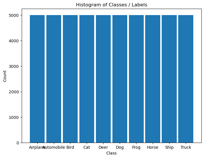
Plot the Data#
# Extract Data

tX = dsTrain.data #<! NumPy Tensor (NDarray)
mX = np.reshape(tX, (tX.shape[0], -1))
vY = dsTrain.targets #<! NumPy Vector
# Plot the Data

hF = PlotMnistImages(mX, vY, numImg, tuImgSize = T_IMG_SIZE)
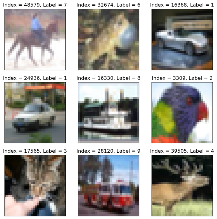
# Histogram of Labels

hA = PlotLabelsHistogram(vY, lClass = L_CLASSES)
plt.show()
(?) If data is converted into grayscale, how would it effect the performance of the classifier? Explain.
You may assume the conversion is done using the mean value of the RGB pixel.
Pre Process Data#
This section normalizes the data to have zero mean and unit variance per channel.
It is required to calculate:
The average pixel value per channel.
The standard deviation per channel.
(#) The values calculated on the train set and applied to both sets.
(#) The the data will be used to pre process the image on loading by the
transformer.(#) There packages which specializes in transforms:
Kornia,Albumentations.
They are commonly used for Data Augmentation at scale.
# Calculate the Standardization Parameters
vMean = np.mean(dsTrain.data / 255.0, axis = (0, 1, 2))
vStd  = np.std(dsVal.data / 255.0, axis = (0, 1, 2))

print('µ =', vMean)
print('σ =', vStd)
µ = [0.49139968 0.48215841 0.44653091]
σ = [0.24665252 0.24289226 0.26159238]
# Update Transformer

oTrnsTrain = TorchVisionTrns.Compose([
    TorchVisionTrns.RandomHorizontalFlip(), #<! Can be done in UINT8 for faster performance
    TorchVisionTrns.AutoAugment(policy = TorchVisionTrns.AutoAugmentPolicy.CIFAR10), #<! Requires `UINT8`
    TorchVisionTrns.ToImage(),
    TorchVisionTrns.ToDtype(torch.float32, scale = True),
    TorchVisionTrns.Normalize(vMean, vStd)
])

oTrnsInfer = TorchVisionTrns.Compose([
    TorchVisionTrns.ToImage(),
    TorchVisionTrns.ToDtype(torch.float32, scale = True),
    TorchVisionTrns.Normalize(vMean, vStd)
])

# Update the DS transformer
dsTrain.transform   = oTrnsTrain
dsVal.transform     = oTrnsInfer
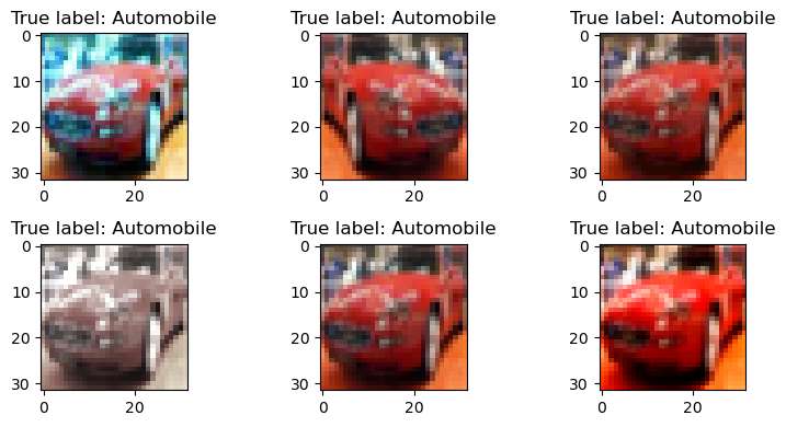
# "Normalized" Image

imgIdx = 5

N, H, W, C = dsTrain.data.shape
hF, vHA = plt.subplots(2, 3, figsize = (8, 4))
vHA = vHA.flat
for hA in vHA:
    mX, valY = dsTrain[imgIdx] #<! Random
    mX = torch.permute(mX, (1, 2, 0))
    hA.imshow(torch.clip(mX * vStd[None, None, :] + vMean[None, None, :], min = 0.0, max = 1.0))
    hA.set_title(f'True label: {L_CLASSES[valY]}')

hF.tight_layout()
Data Loaders#
This section defines the data loaded.
# Data Loader

dlTrain = torch.utils.data.DataLoader(dsTrain, shuffle = True, batch_size = 1 * batchSize, num_workers = 2, drop_last = True, persistent_workers = True)
dlVal   = torch.utils.data.DataLoader(dsVal, shuffle = False, batch_size = 2 * batchSize, num_workers = 2, persistent_workers = True)

# dlTrain = torch.utils.data.DataLoader(dsTrain, shuffle = True, batch_size = 1 * batchSize, num_workers = 0, drop_last = True)
# dlVal   = torch.utils.data.DataLoader(dsVal, shuffle = False, batch_size = 2 * batchSize, num_workers = 0)
# Iterate on the Loader
# The first batch.
tX, vY = next(iter(dlTrain)) #<! PyTorch Tensors

print(f'The batch features dimensions: {tX.shape}')
print(f'The batch labels dimensions: {vY.shape}')
The batch features dimensions: torch.Size([256, 3, 32, 32])
The batch labels dimensions: torch.Size([256])
# Looping
# for ii, (tX, vY) in zip(range(1), dlVal): #<! https://stackoverflow.com/questions/36106712
#     print(f'The batch features dimensions: {tX.shape}')
#     print(f'The batch labels dimensions: {vY.shape}')
Load the Model#
This section loads the model.
The number of outputs is adjusted to match the number of classes in the data.
# Loading a Pre Defined Model
oModel = GenResNetModel(trainedModel = False, numCls = len(L_CLASSES))
# oModel.apply(InitWeightsKaiNorm)
# Model Information - Pre Defined
# Pay attention to the layers name.
torchinfo.summary(oModel, (batchSize, *(T_IMG_SIZE[::-1])), col_names = ['kernel_size', 'output_size', 'num_params'], device = 'cpu', row_settings = ['depth', 'var_names'])
========================================================================================================================
Layer (type (var_name):depth-idx)             Kernel Shape              Output Shape              Param #
========================================================================================================================
ResNet (ResNet)                               --                        [256, 10]                 --
├─Conv2d (conv1): 1-1                         [7, 7]                    [256, 64, 16, 16]         9,408
├─BatchNorm2d (bn1): 1-2                      --                        [256, 64, 16, 16]         128
├─ReLU (relu): 1-3                            --                        [256, 64, 16, 16]         --
├─MaxPool2d (maxpool): 1-4                    3                         [256, 64, 8, 8]           --
├─Sequential (layer1): 1-5                    --                        [256, 64, 8, 8]           --
│    └─BasicBlock (0): 2-1                    --                        [256, 64, 8, 8]           --
│    │    └─Conv2d (conv1): 3-1               [3, 3]                    [256, 64, 8, 8]           36,864
│    │    └─BatchNorm2d (bn1): 3-2            --                        [256, 64, 8, 8]           128
│    │    └─ReLU (relu): 3-3                  --                        [256, 64, 8, 8]           --
│    │    └─Conv2d (conv2): 3-4               [3, 3]                    [256, 64, 8, 8]           36,864
│    │    └─BatchNorm2d (bn2): 3-5            --                        [256, 64, 8, 8]           128
│    │    └─ReLU (relu): 3-6                  --                        [256, 64, 8, 8]           --
│    └─BasicBlock (1): 2-2                    --                        [256, 64, 8, 8]           --
│    │    └─Conv2d (conv1): 3-7               [3, 3]                    [256, 64, 8, 8]           36,864
│    │    └─BatchNorm2d (bn1): 3-8            --                        [256, 64, 8, 8]           128
│    │    └─ReLU (relu): 3-9                  --                        [256, 64, 8, 8]           --
│    │    └─Conv2d (conv2): 3-10              [3, 3]                    [256, 64, 8, 8]           36,864
│    │    └─BatchNorm2d (bn2): 3-11           --                        [256, 64, 8, 8]           128
│    │    └─ReLU (relu): 3-12                 --                        [256, 64, 8, 8]           --
├─Sequential (layer2): 1-6                    --                        [256, 128, 4, 4]          --
│    └─BasicBlock (0): 2-3                    --                        [256, 128, 4, 4]          --
│    │    └─Conv2d (conv1): 3-13              [3, 3]                    [256, 128, 4, 4]          73,728
│    │    └─BatchNorm2d (bn1): 3-14           --                        [256, 128, 4, 4]          256
│    │    └─ReLU (relu): 3-15                 --                        [256, 128, 4, 4]          --
│    │    └─Conv2d (conv2): 3-16              [3, 3]                    [256, 128, 4, 4]          147,456
│    │    └─BatchNorm2d (bn2): 3-17           --                        [256, 128, 4, 4]          256
│    │    └─Sequential (downsample): 3-18     --                        [256, 128, 4, 4]          8,448
│    │    └─ReLU (relu): 3-19                 --                        [256, 128, 4, 4]          --
│    └─BasicBlock (1): 2-4                    --                        [256, 128, 4, 4]          --
│    │    └─Conv2d (conv1): 3-20              [3, 3]                    [256, 128, 4, 4]          147,456
│    │    └─BatchNorm2d (bn1): 3-21           --                        [256, 128, 4, 4]          256
│    │    └─ReLU (relu): 3-22                 --                        [256, 128, 4, 4]          --
│    │    └─Conv2d (conv2): 3-23              [3, 3]                    [256, 128, 4, 4]          147,456
│    │    └─BatchNorm2d (bn2): 3-24           --                        [256, 128, 4, 4]          256
│    │    └─ReLU (relu): 3-25                 --                        [256, 128, 4, 4]          --
├─Sequential (layer3): 1-7                    --                        [256, 256, 2, 2]          --
│    └─BasicBlock (0): 2-5                    --                        [256, 256, 2, 2]          --
│    │    └─Conv2d (conv1): 3-26              [3, 3]                    [256, 256, 2, 2]          294,912
│    │    └─BatchNorm2d (bn1): 3-27           --                        [256, 256, 2, 2]          512
│    │    └─ReLU (relu): 3-28                 --                        [256, 256, 2, 2]          --
│    │    └─Conv2d (conv2): 3-29              [3, 3]                    [256, 256, 2, 2]          589,824
│    │    └─BatchNorm2d (bn2): 3-30           --                        [256, 256, 2, 2]          512
│    │    └─Sequential (downsample): 3-31     --                        [256, 256, 2, 2]          33,280
│    │    └─ReLU (relu): 3-32                 --                        [256, 256, 2, 2]          --
│    └─BasicBlock (1): 2-6                    --                        [256, 256, 2, 2]          --
│    │    └─Conv2d (conv1): 3-33              [3, 3]                    [256, 256, 2, 2]          589,824
│    │    └─BatchNorm2d (bn1): 3-34           --                        [256, 256, 2, 2]          512
│    │    └─ReLU (relu): 3-35                 --                        [256, 256, 2, 2]          --
│    │    └─Conv2d (conv2): 3-36              [3, 3]                    [256, 256, 2, 2]          589,824
│    │    └─BatchNorm2d (bn2): 3-37           --                        [256, 256, 2, 2]          512
│    │    └─ReLU (relu): 3-38                 --                        [256, 256, 2, 2]          --
├─Sequential (layer4): 1-8                    --                        [256, 512, 1, 1]          --
│    └─BasicBlock (0): 2-7                    --                        [256, 512, 1, 1]          --
│    │    └─Conv2d (conv1): 3-39              [3, 3]                    [256, 512, 1, 1]          1,179,648
│    │    └─BatchNorm2d (bn1): 3-40           --                        [256, 512, 1, 1]          1,024
│    │    └─ReLU (relu): 3-41                 --                        [256, 512, 1, 1]          --
│    │    └─Conv2d (conv2): 3-42              [3, 3]                    [256, 512, 1, 1]          2,359,296
│    │    └─BatchNorm2d (bn2): 3-43           --                        [256, 512, 1, 1]          1,024
│    │    └─Sequential (downsample): 3-44     --                        [256, 512, 1, 1]          132,096
│    │    └─ReLU (relu): 3-45                 --                        [256, 512, 1, 1]          --
│    └─BasicBlock (1): 2-8                    --                        [256, 512, 1, 1]          --
│    │    └─Conv2d (conv1): 3-46              [3, 3]                    [256, 512, 1, 1]          2,359,296
│    │    └─BatchNorm2d (bn1): 3-47           --                        [256, 512, 1, 1]          1,024
│    │    └─ReLU (relu): 3-48                 --                        [256, 512, 1, 1]          --
│    │    └─Conv2d (conv2): 3-49              [3, 3]                    [256, 512, 1, 1]          2,359,296
│    │    └─BatchNorm2d (bn2): 3-50           --                        [256, 512, 1, 1]          1,024
│    │    └─ReLU (relu): 3-51                 --                        [256, 512, 1, 1]          --
├─AdaptiveAvgPool2d (avgpool): 1-9            --                        [256, 512, 1, 1]          --
├─Linear (fc): 1-10                           --                        [256, 10]                 5,130
========================================================================================================================
Total params: 11,181,642
Trainable params: 11,181,642
Non-trainable params: 0
Total mult-adds (Units.GIGABYTES): 9.48
========================================================================================================================
Input size (MB): 3.15
Forward/backward pass size (MB): 207.64
Params size (MB): 44.73
Estimated Total Size (MB): 255.51
========================================================================================================================
(?) Does the last (Head) dense layer includes a bias? Explain.
# Model
# Defining a sequential model.

# numChannels = 128

# def BuildModel( nC: int ) -> nn.Module:

#     oModel = nn.Sequential(
#         nn.Identity(),
#         nn.Conv2d(3, nC, 3, padding = 1, bias = False),  nn.BatchNorm2d(nC), nn.ReLU(),                  nn.Dropout2d(0.2),
#         nn.Conv2d(nC, nC, 3, padding = 1, bias = False), nn.BatchNorm2d(nC), nn.ReLU(), nn.MaxPool2d(2), nn.Dropout2d(0.2),

#         ResidualBlock(nC), nn.Dropout2d(0.2),
#         ResidualBlock(nC), nn.Dropout2d(0.2),
#         ResidualBlock(nC), nn.Dropout2d(0.2),
#         ResidualBlock(nC), nn.Dropout2d(0.2),
#         ResidualBlock(nC), nn.Dropout2d(0.2),

#         nn.AdaptiveAvgPool2d(1),
#         nn.Flatten(),
#         nn.Linear(nC, 10)
#     )

#     oModel.apply(InitWeightsKaiNorm)

#     return oModel

# oModel = BuildModel(numChannels)

# torchinfo.summary(oModel, (batchSize, 3, 32, 32), col_names = ['kernel_size', 'output_size', 'num_params'], device = 'cpu')
Train the Model#
This section trains the model.
It compares results with and without Label Smoothing.
(#) The objective is to show how to apply Label Smoothing.
Label Smoothing#
Cross Entropy Loss $\( \ell_{\mathrm{CE}}\left(\boldsymbol{y}_{i},\hat{\boldsymbol{y}}_{i}\right)=-\left\langle \boldsymbol{y}_{i},\log\left(\hat{\boldsymbol{y}}_{i}\right)\right\rangle =-\left\langle \left[\begin{matrix}0\\ 1\\ 0\\ 0 \end{matrix}\right],\log\left(\left[\begin{matrix}0.1\\ 0.75\\ 0.05\\ 0.1 \end{matrix}\right]\right)\right\rangle \)$
Label Smoothing Loss $\( \ell_{\mathrm{LS}}\left(\boldsymbol{y}_{i},\hat{\boldsymbol{y}}_{i}\right)=-\left\langle \left[\begin{matrix}\frac{\epsilon}{3}\\ 1-\epsilon\\ \frac{\epsilon}{3}\\ \frac{\epsilon}{3} \end{matrix}\right],\log\left(\left[\begin{matrix}0.1\\ 0.75\\ 0.05\\ 0.1 \end{matrix}\right]\right)\right\rangle \)$
(#) The value of \(\epsilon\) is a hyper parameter.
(#) PyTorch’s class
CrossEntropyLossimplements Label Smoothing in itslabel_smoothingparameter.
See [PyTorch][Feature Request] Label Smoothing for CrossEntropyLoss.(#) The Label Smoothing loss can be written: \(\ell_{\mathrm{LS}}\left({\color{cyan}\boldsymbol{y}_{i}},{\color{T}\hat{\boldsymbol{y}}_{i}}\right)=-\left\langle {\color{magenta}\boldsymbol{1}\epsilon}+\left(1-{\color{yellow}C}\cdot{\color{magenta}\epsilon}\right){\color{cyan}\boldsymbol{y}_{i}},\log\left({\color{T}\hat{\boldsymbol{y}}_{i}}\right)\right\rangle\).
This can be calculated, by linearity of the Inner Product as 2 CE calculations.
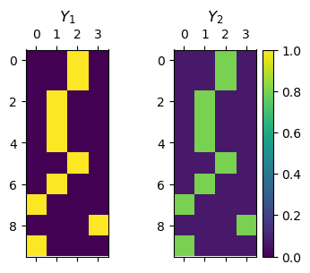
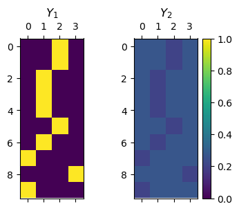
# Label Smoothing by Code

N    = 10                         #<! Number of samples
C    = 4                          #<! Number of classes (Labels)
vIdx = torch.randint(0, C, (N,))  #<! Reference labels

#<! mY1 (One Hot)
mY1 = torch.zeros(N, C)
mY1 = torch.scatter(mY1, 1, torch.unsqueeze(vIdx, 1), 1.0)

#<! mY2 (Smooth)
ϵ   = 0.2
mY2 = torch.full((N, C), ϵ / (C - 1))
mY2 = torch.scatter(mY2, 1, torch.unsqueeze(vIdx, 1), 1 - ϵ)

hF, hA = plt.subplots(1, 2, figsize = (4, 3))
hImg = hA[0].matshow(mY1, vmin = 0, vmax = 1)
hImg = hA[1].matshow(mY2, vmin = 0, vmax = 1)
hA[0].set_title('$Y_1$')
hA[1].set_title('$Y_2$')
hF.colorbar(hImg)
<matplotlib.colorbar.Colorbar at 0x7f20c8328b10>
#<! mY2 (Smooth)
ϵ   = 0.8
mY2 = torch.full((N, C), ϵ / (C - 1))
mY2 = torch.scatter(mY2, 1, torch.unsqueeze(vIdx, 1), 1 - ϵ)

hF, hA = plt.subplots(1, 2, figsize = (4, 3))
hImg = hA[0].matshow(mY1, vmin = 0, vmax = 1)
hImg = hA[1].matshow(mY2, vmin = 0, vmax = 1)
hA[0].set_title('$Y_1$')
hA[1].set_title('$Y_2$')
hF.colorbar(hImg)
<matplotlib.colorbar.Colorbar at 0x7f20c8223250>
# Run Device

runDevice = torch.device('cuda:0' if torch.cuda.is_available() else 'cpu') #<! The 1st CUDA device
# Loss and Score Function
lϵ = [0.0, 0.1]

hS = MulticlassAccuracy(num_classes = len(lClass), average = 'micro')

hS = hS.to(runDevice)
# Training Loop

dModelHist = {}

for ii, ϵ in enumerate(lϵ):
    modelName = f'ϵ={ϵ:3.2f}'
    print(f'Training model: {modelName}')
    hL = nn.CrossEntropyLoss(label_smoothing = ϵ)
    oRunModel = copy.deepcopy(oModel) #<! Transfer model to device
    oRunModel = oRunModel.to(runDevice)
    oOpt = torch.optim.AdamW(oRunModel.parameters(), lr = 1e-3, betas = (0.9, 0.99), weight_decay = 1e-2) #<! Define optimizer
    oSch = torch.optim.lr_scheduler.OneCycleLR(oOpt, max_lr = 5e-2, total_steps = numEpochs)
    _, lTrainLoss, lTrainScore, lValLoss, lValScore, lLearnRate = TrainModel(oRunModel, dlTrain, dlVal, oOpt, numEpochs, hL, hS, oSch = oSch)

    # oSch = torch.optim.lr_scheduler.OneCycleLR(oOpt, max_lr = 5e-2, total_steps = numEpochs * len(dlTrain))
    # _, lTrainLoss, lTrainScore, lValLoss, lValScore, lLearnRate = TrainModelSch(oRunModel, dlTrain, dlVal, oOpt, oSch, numEpochs, hL, hS)
    dModelHist[modelName] = lTrainLoss, lTrainScore, lValLoss, lValScore, lLearnRate
Training model: ϵ=0.00
Epoch    1 / 5 | Train Loss:  1.791 | Val Loss:  1.353 | Train Score:  0.353 | Val Score:  0.512 | Epoch Time: 32.08 | <-- Checkpoint! |
Epoch    2 / 5 | Train Loss:  2.258 | Val Loss:  1.845 | Train Score:  0.160 | Val Score:  0.267 | Epoch Time: 17.37 |
Epoch    3 / 5 | Train Loss:  1.815 | Val Loss:  1.503 | Train Score:  0.311 | Val Score:  0.442 | Epoch Time: 17.07 |
Epoch    4 / 5 | Train Loss:  1.520 | Val Loss:  1.259 | Train Score:  0.443 | Val Score:  0.541 | Epoch Time: 17.39 | <-- Checkpoint! |
Epoch    5 / 5 | Train Loss:  1.427 | Val Loss:  1.225 | Train Score:  0.478 | Val Score:  0.551 | Epoch Time: 17.24 | <-- Checkpoint! |
Training model: ϵ=0.10
Epoch    1 / 5 | Train Loss:  1.899 | Val Loss:  1.600 | Train Score:  0.358 | Val Score:  0.507 | Epoch Time: 17.53 | <-- Checkpoint! |
Epoch    2 / 5 | Train Loss:  2.309 | Val Loss:  2.068 | Train Score:  0.145 | Val Score:  0.201 | Epoch Time: 17.17 |
Epoch    3 / 5 | Train Loss:  1.991 | Val Loss:  1.819 | Train Score:  0.270 | Val Score:  0.369 | Epoch Time: 17.52 |
Epoch    4 / 5 | Train Loss:  1.793 | Val Loss:  1.574 | Train Score:  0.389 | Val Score:  0.502 | Epoch Time: 17.94 |
Epoch    5 / 5 | Train Loss:  1.710 | Val Loss:  1.555 | Train Score:  0.434 | Val Score:  0.511 | Epoch Time: 17.88 | <-- Checkpoint! |
# Plot Training Phase

hF, vHa = plt.subplots(nrows = 1, ncols = 3, figsize = (18, 5))
vHa = np.ravel(vHa)

for modelKey in dModelHist:
    hA = vHa[0]
    hA.plot(dModelHist[modelKey][0], lw = 2, label = f'Train {modelKey}')
    hA.plot(dModelHist[modelKey][2], lw = 2, label = f'Validation {modelKey}')
    hA.set_title('Cross Entropy Loss')
    hA.set_xlabel('Epoch')
    hA.set_ylabel('Loss')
    hA.legend()

    hA = vHa[1]
    hA.plot(dModelHist[modelKey][1], lw = 2, label = f'Train {modelKey}')
    hA.plot(dModelHist[modelKey][3], lw = 2, label = f'Validation {modelKey}')
    hA.set_title('Accuracy Score')
    hA.set_xlabel('Epoch')
    hA.set_ylabel('Score')
    hA.legend()

    hA = vHa[2]
    hA.plot(lLearnRate, lw = 2, label = f'{modelKey}')
    hA.set_title('Learn Rate Scheduler')
    hA.set_xlabel('Iteration')
    hA.set_ylabel('Learn Rate')
    hA.legend()
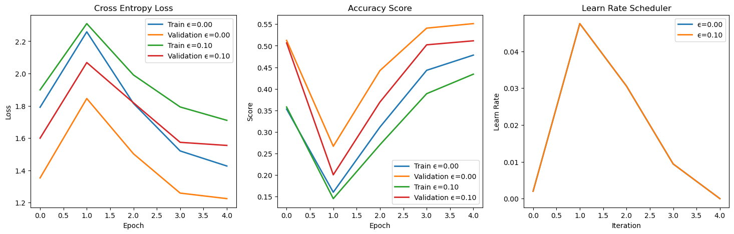
(?) Is the loss landscape comparable between the 2 training phases?