PCA Brest Cancer

PCA Brest Cancer#

UnSupervised Learning - Dimensionality Reduction - Principal Component Analysis#

Notebook by:

Royi Avital RoyiAvital@fixelalgorithms.com

Revision History#

Version	Date	User	Content / Changes
1.0.000	13/04/2024	Royi Avital	First version

# Import Packages

# General Tools
import numpy as np
import scipy as sp
import pandas as pd

# Machine Learning
from sklearn.datasets import load_breast_cancer
from sklearn.decomposition import PCA
from sklearn.feature_selection import SequentialFeatureSelector
from sklearn.linear_model import LogisticRegression
from sklearn.model_selection import cross_val_score
from sklearn.pipeline import Pipeline
from sklearn.preprocessing import StandardScaler

# Miscellaneous
import math
import os
from platform import python_version
import random
import timeit

# Typing
from typing import Callable, Dict, List, Optional, Self, Set, Tuple, Union

# Visualization
import matplotlib as mpl
import matplotlib.pyplot as plt
import seaborn as sns

# Jupyter
from IPython import get_ipython
from IPython.display import Image
from IPython.display import display
from ipywidgets import Dropdown, FloatSlider, interact, IntSlider, Layout, SelectionSlider
from ipywidgets import interact

Notations#

(?) Question to answer interactively.
(!) Simple task to add code for the notebook.
(@) Optional / Extra self practice.
(#) Note / Useful resource / Food for thought.

Code Notations:

someVar    = 2; #<! Notation for a variable
vVector    = np.random.rand(4) #<! Notation for 1D array
mMatrix    = np.random.rand(4, 3) #<! Notation for 2D array
tTensor    = np.random.rand(4, 3, 2, 3) #<! Notation for nD array (Tensor)
tuTuple    = (1, 2, 3) #<! Notation for a tuple
lList      = [1, 2, 3] #<! Notation for a list
dDict      = {1: 3, 2: 2, 3: 1} #<! Notation for a dictionary
oObj       = MyClass() #<! Notation for an object
dfData     = pd.DataFrame() #<! Notation for a data frame
dsData     = pd.Series() #<! Notation for a series
hObj       = plt.Axes() #<! Notation for an object / handler / function handler

Code Exercise#

Single line fill

vallToFill = ???

Multi Line to Fill (At least one)

# You need to start writing
????

Section to Fill

#===========================Fill This===========================#
# 1. Explanation about what to do.
# !! Remarks to follow / take under consideration.
mX = ???

???
#===============================================================#

# Configuration
# %matplotlib inline

seedNum = 512
np.random.seed(seedNum)
random.seed(seedNum)

# Matplotlib default color palette
lMatPltLibclr = ['#1f77b4', '#ff7f0e', '#2ca02c', '#d62728', '#9467bd', '#8c564b', '#e377c2', '#7f7f7f', '#bcbd22', '#17becf']
# sns.set_theme() #>! Apply SeaBorn theme

runInGoogleColab = 'google.colab' in str(get_ipython())

# Constants

FIG_SIZE_DEF    = (8, 8)
ELM_SIZE_DEF    = 50
CLASS_COLOR     = ('b', 'r')
EDGE_COLOR      = 'k'
MARKER_SIZE_DEF = 10
LINE_WIDTH_DEF  = 2

# Courses Packages
import sys
sys.path.append('../')
sys.path.append('../../')
sys.path.append('../../../')
from utils.DataVisualization import PlotScatterData

# General Auxiliary Functions

hOrdinalNum = lambda n: '%d%s' % (n, 'tsnrhtdd'[(((math.floor(n / 10) %10) != 1) * ((n % 10) < 4) * (n % 10))::4])

Dimensionality Reduction by PCA#

In this exercise we’ll use the PCA approach for dimensionality reduction within a pipeline.

This exercise introduces:

Working with the Breast Cancer Wisconsin Data Set.
Combine the PCA as a transformer in a pipeline with a linear classifier to predict the binary class of the data.
Select the best features using a sequential approach.

The objective is to optimize the feature selection in order to get the best classification accuracy.

(#) PCA is the most basic dimensionality reduction operator.
(#) The PCA output is a linear combination of the input.

# Parameters

# Data

# Model
numComp  = 2
paramC   = 1
numKFold = 5
numFeat  = 5

Generate / Load Data#

In this notebook we’ll use the Breast Cancer Wisconsin Data Set.

Features are computed from a digitized image of a fine needle aspirate (FNA) of a breast mass.

# Load Data

mX, vY   = load_breast_cancer(return_X_y = True)
dfX, dsY = load_breast_cancer(return_X_y = True, as_frame = True)

print(f'The features data shape: {mX.shape}')

The features data shape: (569, 30)

# Merge Label Data
dfData = dfX.copy()
dfData['Label'] = pd.Categorical(dsY)

dfData

	mean radius	mean texture	mean perimeter	mean area	mean smoothness	mean compactness	mean concavity	mean concave points	mean symmetry	mean fractal dimension	...	worst texture	worst perimeter	worst area	worst smoothness	worst compactness	worst concavity	worst concave points	worst symmetry	worst fractal dimension	Label
0	17.99	10.38	122.80	1001.0	0.11840	0.27760	0.30010	0.14710	0.2419	0.07871	...	17.33	184.60	2019.0	0.16220	0.66560	0.7119	0.2654	0.4601	0.11890	0
1	20.57	17.77	132.90	1326.0	0.08474	0.07864	0.08690	0.07017	0.1812	0.05667	...	23.41	158.80	1956.0	0.12380	0.18660	0.2416	0.1860	0.2750	0.08902	0
2	19.69	21.25	130.00	1203.0	0.10960	0.15990	0.19740	0.12790	0.2069	0.05999	...	25.53	152.50	1709.0	0.14440	0.42450	0.4504	0.2430	0.3613	0.08758	0
3	11.42	20.38	77.58	386.1	0.14250	0.28390	0.24140	0.10520	0.2597	0.09744	...	26.50	98.87	567.7	0.20980	0.86630	0.6869	0.2575	0.6638	0.17300	0
4	20.29	14.34	135.10	1297.0	0.10030	0.13280	0.19800	0.10430	0.1809	0.05883	...	16.67	152.20	1575.0	0.13740	0.20500	0.4000	0.1625	0.2364	0.07678	0
...	...	...	...	...	...	...	...	...	...	...	...	...	...	...	...	...	...	...	...	...	...
564	21.56	22.39	142.00	1479.0	0.11100	0.11590	0.24390	0.13890	0.1726	0.05623	...	26.40	166.10	2027.0	0.14100	0.21130	0.4107	0.2216	0.2060	0.07115	0
565	20.13	28.25	131.20	1261.0	0.09780	0.10340	0.14400	0.09791	0.1752	0.05533	...	38.25	155.00	1731.0	0.11660	0.19220	0.3215	0.1628	0.2572	0.06637	0
566	16.60	28.08	108.30	858.1	0.08455	0.10230	0.09251	0.05302	0.1590	0.05648	...	34.12	126.70	1124.0	0.11390	0.30940	0.3403	0.1418	0.2218	0.07820	0
567	20.60	29.33	140.10	1265.0	0.11780	0.27700	0.35140	0.15200	0.2397	0.07016	...	39.42	184.60	1821.0	0.16500	0.86810	0.9387	0.2650	0.4087	0.12400	0
568	7.76	24.54	47.92	181.0	0.05263	0.04362	0.00000	0.00000	0.1587	0.05884	...	30.37	59.16	268.6	0.08996	0.06444	0.0000	0.0000	0.2871	0.07039	1

569 rows × 31 columns

Exploratory Data Analysis (EDA)#

Correlation Matrix#

The correlation matrix is appropriate tool to filter features which are highly correlated.
It is less effective for feature selection.

# Correlation Matrix
hF, hA = plt.subplots(figsize = (14, 14))
dfData['Label'] = pd.to_numeric(dfData['Label'])
mC = dfData.corr(method = 'pearson')
sns.heatmap(mC.abs(), cmap = 'coolwarm', annot = True, fmt = '2.1f', ax = hA)

plt.show()

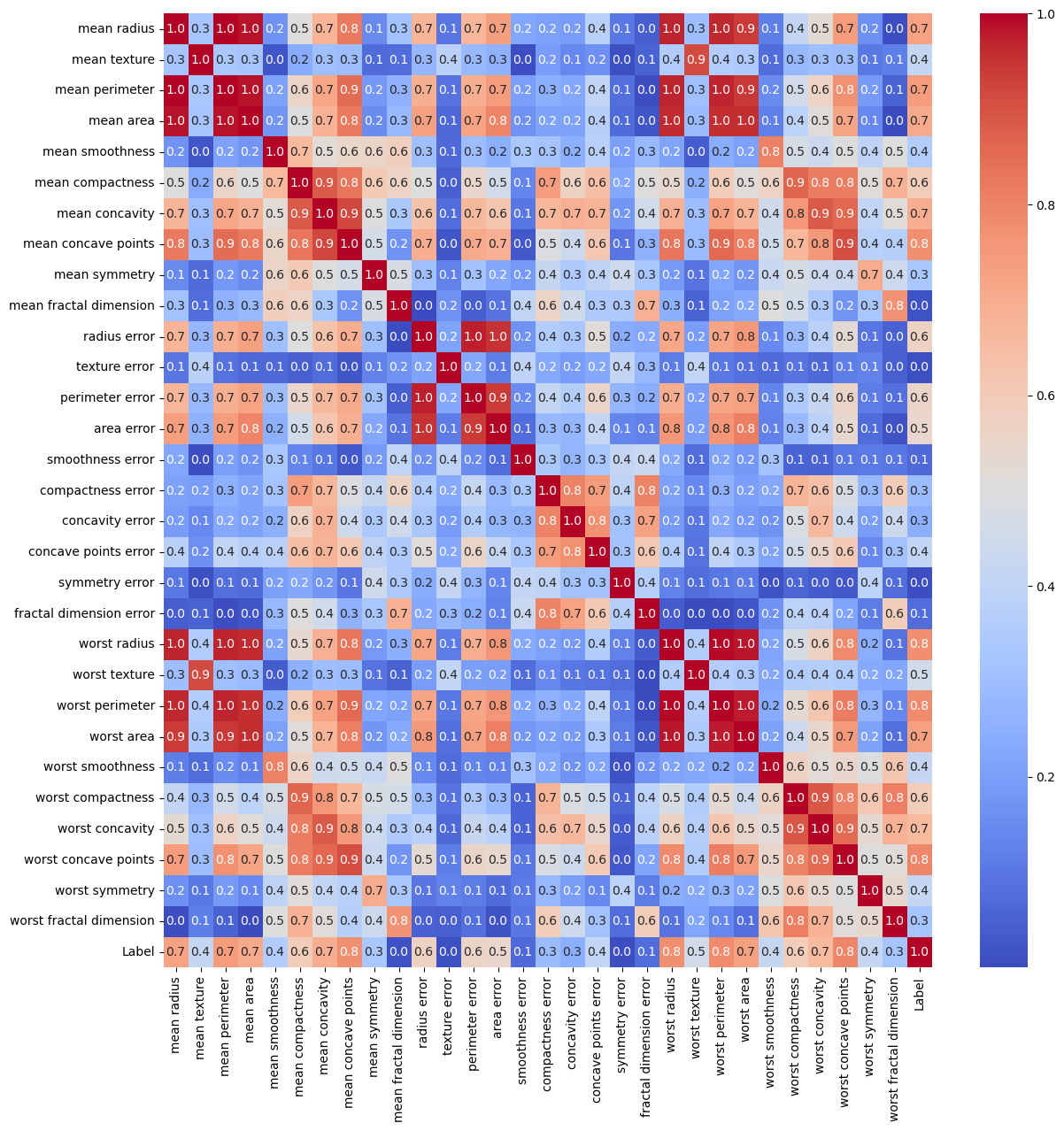
../../../../_images/fde254ce177228e93d9fb643f64087e5edc73e243b47b6c8ce41ba0f591610d2.png

(?) Are there redundant features? Think in the context of PCA.

Pre Processing#

# Standardize the Data
# Make each feature: Zero Mean, Unit Variance.

#===========================Fill This===========================#
# 1. Construct the standard scaler.
# 2. Apply it to data.
?????
#===============================================================#

Object `???` not found.

Applying Dimensionality Reduction - PCA#

The common usage for Dimensionality Reduction:

Noise Reduction (Increase SNR).
Compute Efficiency.
Visualization.
Feature Engineering Step (Usually as Manifold Learning).

# Applying the PCA Model

#===========================Fill This===========================#
# 1. Construct the PCA model.
# 2. Apply it to data.
oPCA = ???
mZ   = ???
#===============================================================#

  Cell In[22], line 6
    oPCA = ???
           ^
SyntaxError: invalid syntax

Plot Data in 2D#

One useful use of Dimensionality Reduction is visualizing high dimensional data.

# Plot the 2D Result

hA = PlotScatterData(mZ, vY)

(#) The optimal Dimensionality Reduction is the perfect feature engineering.
(#) Dimensionality Reduction is usually used as a step in pipeline.
(?) Can we use Clustering as a dimensionality reduction?

Pipeline with PCA#

In this section we’ll build a simple pipeline:

Apply PCA with 2 components.
Apply Linear Classifier.

We’ll tweak the model with selecting the best features as an input to the PCA.
To do that we’ll use the SequentialFeatureSelector object of SciKit Learn.

Selecting features sequentially is a compute intensive operation.
Hence we can use when the following assumptions hold:

The number of features is modest (< 100).
The cross validation loop (The estimator / pipeline fit() and predict()) process is fast.

Of course the time budget and computing budget are also main factors.

# Building the Pipeline

#===========================Fill This===========================#
# 1. Construct a pipeline with the first operation being PCA and then Logistic Regressor.
# 2. Set the `n_components` and `C` hyper parameters.
oPipeCls = Pipeline([('PCA', PCA(n_components = ???)), ('Classifier', LogisticRegression(C = ???))])
#===============================================================#

# Base Line Score

#===========================Fill This===========================#
# 1. Compute the base line score (Accuracy) as the mean of the output of `cross_val_score`.
scoreAccBase = ???
#===============================================================#

(?) What are the issues with cross_val_score? Think the cases where folds are not evenly divided or the score is not linear.

# Selecting the Features

#===========================Fill This===========================#
# 1. Construct the `SequentialFeatureSelector` object by setting the (Use the parameters defined above):
#   - `estimator`.
#   - `n_features_to_select`.
#   - `direction`.
#   - `cv`.
# 2. Fit it to data.
# !! Set `direction` wisely. Pay attention that `PCA` with `numComp` components requires at least `numComp` features (Assuming `numSamples` > `numFeatures`).
oFeatSelector = SequentialFeatureSelector(estimator = ???, n_features_to_select = ???, direction = ???, cv = ???)
oFeatSelector = ???
#===============================================================#

# Extracting Selected Features
vSelectedFeat = oFeatSelector.get_support()

(?) How should we use the above results in production?

# Optimized Score

#===========================Fill This===========================#
# 1. Compute the optimized score (Accuracy) as the mean of the output of `cross_val_score`.
# 2. Select the features from `vSelectedFeat`.
scoreAccOpt = ???
#===============================================================#

# Comparing Results

print(f'The base line score (Accuracy): {scoreAccBase:0.2%}.')
print(f'The optimized score (Accuracy): {scoreAccOpt:0.2%}.')

# The Selected Features

dfX.columns[vSelectedFeat]

(?) Look at the correlation matrix, how correlated are the selected features relative to other?
(?) Given the pipeline above, can we think on a more efficient way to select features?
(@) Optimize all hyper parameters of the model: n_features_to_select, n_components and C.