Gaussian Mixture Models (GMM)#
Notebook by:
Royi Avital RoyiAvital@fixelalgorithms.com
Revision History#
Version |
Date |
User |
Content / Changes |
|---|---|---|---|
1.0.000 |
13/04/2024 |
Royi Avital |
First version |
![]()
# Import Packages

# General Tools
import numpy as np
import scipy as sp
import pandas as pd

# Machine Learning
from sklearn.datasets import load_iris, make_blobs
from sklearn.mixture import GaussianMixture
from sklearn.model_selection import StratifiedKFold

# Miscellaneous
import math
import os
from platform import python_version
import random
import timeit

# Typing
from typing import Callable, Dict, List, Optional, Self, Set, Tuple, Union

# Visualization
import matplotlib as mpl
import matplotlib.pyplot as plt
import seaborn as sns

# Jupyter
from IPython import get_ipython
from IPython.display import Image
from IPython.display import display
from ipywidgets import Dropdown, FloatSlider, interact, IntSlider, Layout, SelectionSlider
from ipywidgets import interact
Notations#
(?) Question to answer interactively.
(!) Simple task to add code for the notebook.
(@) Optional / Extra self practice.
(#) Note / Useful resource / Food for thought.
Code Notations:
someVar    = 2; #<! Notation for a variable
vVector    = np.random.rand(4) #<! Notation for 1D array
mMatrix    = np.random.rand(4, 3) #<! Notation for 2D array
tTensor    = np.random.rand(4, 3, 2, 3) #<! Notation for nD array (Tensor)
tuTuple    = (1, 2, 3) #<! Notation for a tuple
lList      = [1, 2, 3] #<! Notation for a list
dDict      = {1: 3, 2: 2, 3: 1} #<! Notation for a dictionary
oObj       = MyClass() #<! Notation for an object
dfData     = pd.DataFrame() #<! Notation for a data frame
dsData     = pd.Series() #<! Notation for a series
hObj       = plt.Axes() #<! Notation for an object / handler / function handler
Code Exercise#
Single line fill
vallToFill = ???
Multi Line to Fill (At least one)
# You need to start writing
????
Section to Fill
#===========================Fill This===========================#
# 1. Explanation about what to do.
# !! Remarks to follow / take under consideration.
mX = ???

???
#===============================================================#
# Configuration
# %matplotlib inline

seedNum = 512
np.random.seed(seedNum)
random.seed(seedNum)

# Matplotlib default color palette
lMatPltLibclr = ['#1f77b4', '#ff7f0e', '#2ca02c', '#d62728', '#9467bd', '#8c564b', '#e377c2', '#7f7f7f', '#bcbd22', '#17becf']
# sns.set_theme() #>! Apply SeaBorn theme

runInGoogleColab = 'google.colab' in str(get_ipython())

# GMM Warnings
from sklearn.exceptions import ConvergenceWarning
import warnings
warnings.filterwarnings('ignore', category = ConvergenceWarning) #<! Suppress GMM convergence warning
# Constants

FIG_SIZE_DEF    = (8, 8)
ELM_SIZE_DEF    = 50
CLASS_COLOR     = ('b', 'r')
EDGE_COLOR      = 'k'
MARKER_SIZE_DEF = 10
LINE_WIDTH_DEF  = 2
# Courses Packages
import sys
sys.path.append('../')
sys.path.append('../../')
sys.path.append('../../../')
from utils.DataVisualization import PlotScatterData
# General Auxiliary Functions

def GenRotMatrix( θ: float ) -> np.ndarray:
    thetaAng = np.radians(θ) #<! Convert Degrees -> Radians
    cosVal, sinVal = np.cos(thetaAng), np.sin(thetaAng)

    mR = np.array([[cosVal, -sinVal], [sinVal, cosVal]])

    return mR


def PlotGmm( mX: np.ndarray, numClusters: int, numIter: int, initMethod: str = 'random', hA: Optional[plt.Axes] = None, figSize: Tuple[int, int] = FIG_SIZE_DEF, markerSize: int = MARKER_SIZE_DEF ) -> plt.Axes:

    if hA is None:
        hF, hA = plt.subplots(figsize = figSize)
    else:
        hF = hA.get_figure()

    oGmm = GaussianMixture(n_components = numClusters, max_iter = numIter, init_params = initMethod, random_state = 0)
    oGmm = oGmm.fit(mX)

    vIdx    = oGmm.predict(mX)
    mMu     = oGmm.means_

    hS = hA.scatter(mX[:, 0], mX[:, 1], s = ELM_SIZE_DEF, c = vIdx, edgecolor = EDGE_COLOR)
    hA.plot(mMu[:,0], mMu[:, 1], '.r', markersize = 20)
    for ii in range(numClusters):
        mC = oGmm.covariances_[ii]
        v, w = np.linalg.eigh(mC)
        u = w[0] / np.linalg.norm(w[0])
        angle = np.arctan2(u[1], u[0])
        angle = 180 * angle / np.pi  #<! Convert to degrees
        v = 2.0 * np.sqrt(2.0) * np.sqrt(v)
        ell = mpl.patches.Ellipse(oGmm.means_[ii, :], v[0], v[1], angle = 180 + angle, color = hS.cmap(ii / (numClusters - 1)))
        ell.set_clip_box(hA.bbox)
        ell.set_alpha(0.5)
        hA.add_artist(ell)
    hA.axis('equal')
    hA.axis([-10, 10, -10, 10])
    hA.set_xlabel('${{x}}_{{1}}$')
    hA.set_ylabel('${{x}}_{{2}}$')
    hA.set_title(f'K-Means Clustering, AIC = {oGmm.aic(mX)}, BIC = {oGmm.bic(mX)}')

    return hA
Clustering by GMM#
This notebook demonstrates the use the GMM for clustering.
The GMM can be thought as extension to K-Means with soft assignment and support for non equal and non isotropic blobs.
As the GMM is a combination of Gaussian Distributions its “atom” is the ellipsoid.
(#) With some data scaling the K-Means can also support non isotropic data.
# Parameters

# Data Generation
vNumSamples = [50, 150, 500, 100]
mMu         = [[0, 0], [2, 2], [-2.5, -2.5], [-4, 4]]
vClusterStd = [0.1, 1, 2, 1.5]

# Model
Generate / Load Data#
A set of anisotropic blobs.
# Generate Data

mX, vL = make_blobs(n_samples = vNumSamples, n_features = 2, centers = mMu, cluster_std = vClusterStd)
numSamples  = mX.shape[0]

print(f'The features data shape: {mX.shape}')
The features data shape: (800, 2)
(?) Where are the labels in this case?
Plot Data#
# Plot the Data

hF, hA = plt.subplots(figsize = (8, 8))

hA = PlotScatterData(mX, vL, hA = hA)
hA.set_title('Set of Anisotropic Blobs')

plt.show()
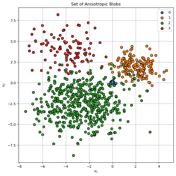
(?) Are there points which are confusing in their labeling?
Cluster Data by Expectation Maximization (EM) for the GMM Model#
Step I:
Assume fixed parameters \(\left\{ w_{k}\right\}\), \(\left\{ \boldsymbol{\mu}_{k}\right\}\) and \(\left\{ \boldsymbol{\Sigma}_{k}\right\}\).
Compute the probability that \(\boldsymbol{x}_{i}\) belong to \(\mathcal{D}_{k}\):
Step II: Assume fixed probabilities \(P_{X_{i}}\left(k\right)\).
Update the parameters \(\left\{ w_{k}\right\}\), \(\left\{ \boldsymbol{\mu}_{k}\right\}\) and \(\left\{ \boldsymbol{\Sigma}_{k}\right\}\) by:
Step III:
Check for convergence (Change in assignments / location of the center). If not, go to Step I.
(#) The GMM is implemented by the
GaussianMixtureclass in SciKit Learn.
(?) Think of the convergence check options. Think of the cases of large data set vs. small data set.
(#) A useful initialization for the GMM is using few K-Means iterations.
# Visualization Wrapper Function
hPlotGmm = lambda numClusters, numIter, initMethod: PlotGmm(mX, numClusters = numClusters, numIter = numIter, initMethod = initMethod, figSize = (7, 7))
# Interactive Visualization

numClustersSlider = IntSlider(min = 2, max = 10, step = 1, value = 3, layout = Layout(width = '30%'))
numIterSlider = IntSlider(min = 1, max = 100, step = 1, value = 1, layout = Layout(width = '30%'))
if runInGoogleColab:
    initMethodDropdown = Dropdown(description = 'Initialization Method', options = [('K-Means', 'kmeans')], value = 'kmeans')
else:
    initMethodDropdown = Dropdown(description = 'Initialization Method', options = [('K-Means', 'kmeans'), ('Random', 'random_from_data'), ('K-Means++', 'k-means++')], value = 'random_from_data')
interact(hPlotGmm, numClusters = numClustersSlider, numIter = numIterSlider, initMethod = initMethodDropdown)

plt.show()
Optimizing the Number of Clusters#
In order to set the number of clusters automatically one can use:
The Elbow Method of the K-Means.
The Silhouette Score.
The Akaike Information Criterion (AIC) and Bayesian Information Criterion (BIC) measures.
The AIC and BIC measures the performance of the model in prediction vs. its complexity.
They try to find the optimal point between model complexity and performance (Bias <-> Variance / Underfit <-> Overfit).
The GaussianMixture has the aic() and bic() methods.
(#) One may use the AIC and BIC in the K-Means context as well.
# Analysis of Performance by AIC and BIC
lK = list(range(1, 10))
numK = len(lK)
vAic = np.full(shape = numK, fill_value = np.nan)
vBic = np.full(shape = numK, fill_value = np.nan)

for ii, valK in enumerate(lK):
    oGmm = GaussianMixture(n_components = valK, max_iter = 2_000, init_params = 'kmeans', random_state = 0)
    oGmm = oGmm.fit(mX)
    vAic[ii] = oGmm.aic(mX)
    vBic[ii] = oGmm.bic(mX)
# Plot Results

hF, hA = plt.subplots(figsize = (8, 8))
hA.plot(lK, vAic, lw = 2, label = 'AIC')
hA.plot(lK, vBic, lw = 2, label = 'BIC')
hA.set_xlabel('Number of Clusters (K)')
hA.set_ylabel('Information Criteria')
hA.set_title('Information Criteria per K')
hA.legend();
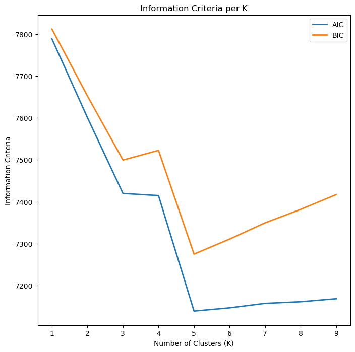
(#) The optimal value is the minimum which is the point where the performance per complexity is maximized.
(#) In general, it might be best to use AIC and BIC together in model selection.
The main differences between the two is that BIC penalizes model complexity more heavily. If BIC points to a three clusters model and AIC points to a five clusters model, it makes sense to select from models with 3, 4 and 5 latent classes.(#) In cases there is no minimum point, it is useful to look at the maximum gradient (Similar to the Elbow Trick). See Gaussian Mixture Model Clusterization: How to Select the Number of Components.
(#) Additional readings: GMM Algorithm, Choosing between AIC and BIC.
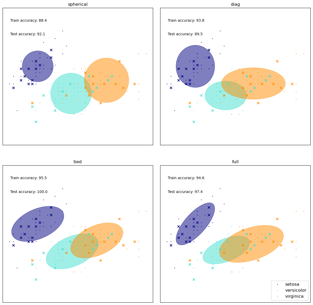
Different Covariance Matrix Assumptions#
We’ll watch the effect of the covariance matrix on the results.
# From SciKit Learn

colors = ["navy", "turquoise", "darkorange"]


def make_ellipses(gmm, ax):
    for n, color in enumerate(colors):
        if gmm.covariance_type == "full":
            covariances = gmm.covariances_[n][:2, :2]
        elif gmm.covariance_type == "tied":
            covariances = gmm.covariances_[:2, :2]
        elif gmm.covariance_type == "diag":
            covariances = np.diag(gmm.covariances_[n][:2])
        elif gmm.covariance_type == "spherical":
            covariances = np.eye(gmm.means_.shape[1]) * gmm.covariances_[n]
        v, w = np.linalg.eigh(covariances)
        u = w[0] / np.linalg.norm(w[0])
        angle = np.arctan2(u[1], u[0])
        angle = 180 * angle / np.pi  # convert to degrees
        v = 2.0 * np.sqrt(2.0) * np.sqrt(v)
        ell = mpl.patches.Ellipse(
            gmm.means_[n, :2], v[0], v[1], angle = 180 + angle, color=color
        )
        ell.set_clip_box(ax.bbox)
        ell.set_alpha(0.5)
        ax.add_artist(ell)
        ax.set_aspect("equal", "datalim")


iris = load_iris()

# Break up the dataset into non-overlapping training (75%) and testing
# (25%) sets.
skf = StratifiedKFold(n_splits=4)
# Only take the first fold.
train_index, test_index = next(iter(skf.split(iris.data, iris.target)))


X_train = iris.data[train_index]
y_train = iris.target[train_index]
X_test = iris.data[test_index]
y_test = iris.target[test_index]

n_classes = len(np.unique(y_train))

# Try GMMs using different types of covariances.
estimators = {
    cov_type: GaussianMixture(
        n_components=n_classes, covariance_type=cov_type, max_iter=20, random_state=0
    )
    for cov_type in ["spherical", "diag", "tied", "full"]
}

n_estimators = len(estimators)

plt.figure(figsize=(12, 12))
plt.subplots_adjust(
    bottom=0.01, top=0.95, hspace=0.15, wspace=0.05, left=0.01, right=0.99
)


for index, (name, estimator) in enumerate(estimators.items()):
    # Since we have class labels for the training data, we can
    # initialize the GMM parameters in a supervised manner.
    estimator.means_init = np.array(
        [X_train[y_train == i].mean(axis=0) for i in range(n_classes)]
    )

    # Train the other parameters using the EM algorithm.
    estimator.fit(X_train)

    h = plt.subplot(2, n_estimators // 2, index + 1)
    make_ellipses(estimator, h)

    for n, color in enumerate(colors):
        data = iris.data[iris.target == n]
        plt.scatter(
            data[:, 0], data[:, 1], s=0.8, color=color, label=iris.target_names[n]
        )
    # Plot the test data with crosses
    for n, color in enumerate(colors):
        data = X_test[y_test == n]
        plt.scatter(data[:, 0], data[:, 1], marker="x", color=color)

    y_train_pred = estimator.predict(X_train)
    train_accuracy = np.mean(y_train_pred.ravel() == y_train.ravel()) * 100
    plt.text(0.05, 0.9, "Train accuracy: %.1f" % train_accuracy, transform=h.transAxes)

    y_test_pred = estimator.predict(X_test)
    test_accuracy = np.mean(y_test_pred.ravel() == y_test.ravel()) * 100
    plt.text(0.05, 0.8, "Test accuracy: %.1f" % test_accuracy, transform=h.transAxes)

    plt.xticks(())
    plt.yticks(())
    plt.title(name)

plt.legend(scatterpoints = 1, loc = "lower right", prop = dict(size = 12))


plt.show()