Dimensionality Reduction - Kernel PCA

Notebook by:

• Royi Avital RoyiAvital@fixelalgorithms.com

Revision History

Version	Date	User	Content / Changes
1.0.000	13/04/2024	Royi Avital	First version

# Import Packages

# General Tools
import numpy as np
import scipy as sp
import pandas as pd

# Machine Learning
from sklearn.datasets import make_circles
from sklearn.decomposition import KernelPCA, PCA

# Miscellaneous
import math
import os
from platform import python_version
import random
import timeit

# Typing
from typing import Callable, Dict, List, Optional, Self, Set, Tuple, Union

# Visualization
import matplotlib as mpl
import matplotlib.pyplot as plt
import seaborn as sns

# Jupyter
from IPython import get_ipython
from IPython.display import Image
from IPython.display import display
from ipywidgets import Dropdown, FloatSlider, interact, IntSlider, Layout, SelectionSlider
from ipywidgets import interact

Notations

• (?) Question to answer interactively.

• (!) Simple task to add code for the notebook.

• (@) Optional / Extra self practice.

• (#) Note / Useful resource / Food for thought.

Code Notations:

someVar    = 2; #<! Notation for a variable
vVector    = np.random.rand(4) #<! Notation for 1D array
mMatrix    = np.random.rand(4, 3) #<! Notation for 2D array
tTensor    = np.random.rand(4, 3, 2, 3) #<! Notation for nD array (Tensor)
tuTuple    = (1, 2, 3) #<! Notation for a tuple
lList      = [1, 2, 3] #<! Notation for a list
dDict      = {1: 3, 2: 2, 3: 1} #<! Notation for a dictionary
oObj       = MyClass() #<! Notation for an object
dfData     = pd.DataFrame() #<! Notation for a data frame
dsData     = pd.Series() #<! Notation for a series
hObj       = plt.Axes() #<! Notation for an object / handler / function handler

Code Exercise

• Single line fill

vallToFill = ???

• Multi Line to Fill (At least one)

# You need to start writing
????

• Section to Fill

#===========================Fill This===========================#
# 1. Explanation about what to do.
# !! Remarks to follow / take under consideration.
mX = ???

???
#===============================================================#

# Configuration
# %matplotlib inline

seedNum = 512
np.random.seed(seedNum)
random.seed(seedNum)

# Matplotlib default color palette
lMatPltLibclr = ['#1f77b4', '#ff7f0e', '#2ca02c', '#d62728', '#9467bd', '#8c564b', '#e377c2', '#7f7f7f', '#bcbd22', '#17becf']
# sns.set_theme() #>! Apply SeaBorn theme

runInGoogleColab = 'google.colab' in str(get_ipython())

# Constants

FIG_SIZE_DEF    = (8, 8)
ELM_SIZE_DEF    = 50
CLASS_COLOR     = ('b', 'r')
EDGE_COLOR      = 'k'
MARKER_SIZE_DEF = 10
LINE_WIDTH_DEF  = 2

# Courses Packages
import sys
sys.path.append('../')
sys.path.append('../../')
sys.path.append('../../../')
from utils.DataVisualization import PlotScatterData

# General Auxiliary Functions

Dimensionality Reduction by Kernel - PCA

The Kernel PCA is a specific case of applying non linear transformation on the features and then applying the PCA transform.
Utilizing the Kernel Trick in the PCA framework allows an efficient computation of the transforms which can be defined by a kernel.

This notebook demonstrates a simple use case of the Kernel PCA.

# Parameters

# Data 
numCircles0 = 350
numCircles1 = 350
noiseLevel  = 0.01

# Model
kernelType  = 'rbf'
γ           = 10.0
α           = 0.1
numComp     = 2

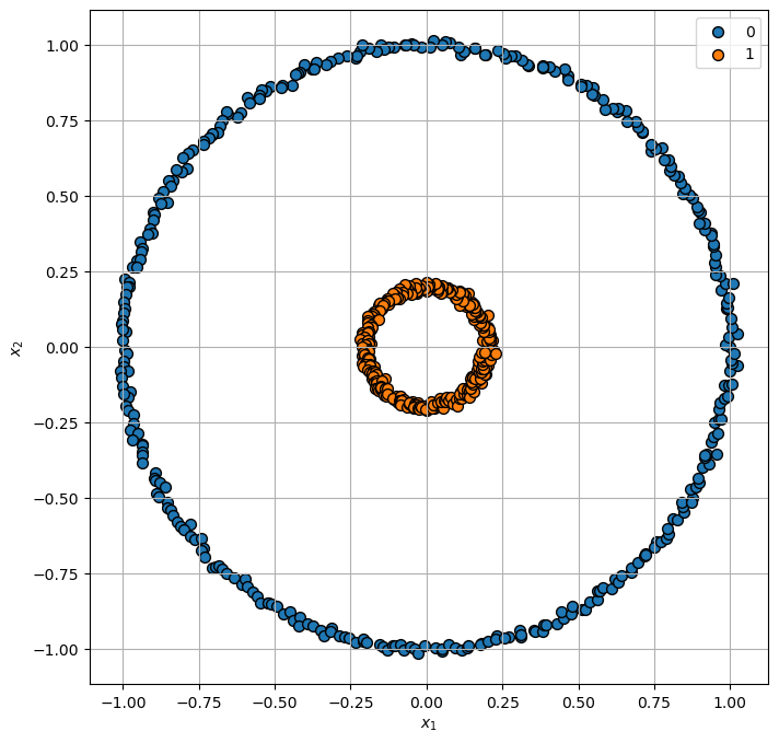
Generate / Load Data

Generating concentric circles.

# Generate Data
numCircles = numCircles0 + numCircles1
mX, vY     = make_circles((numCircles0, numCircles1), factor = 0.2, shuffle = False, noise = noiseLevel, random_state = seedNum)

numSamples = np.size(mX, 0)

print(f'The features data shape: {mX.shape}')
print(f'The labels data shape: {vY.shape}')

The features data shape: (700, 2)
The labels data shape: (700,)

Plot Data

# Plot the Data

hF, hA = plt.subplots(figsize = (8, 8))
hA = PlotScatterData(mX, vY, hA)

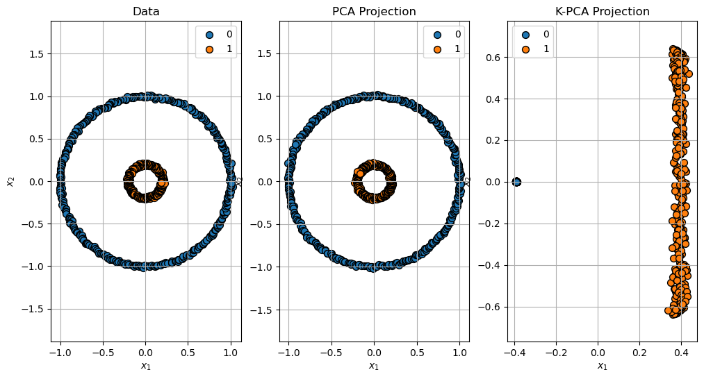
Applying Dimensionality Reduction - Kernel PCA

The Kernel-PCA is usually a framework used by other facilitators (MDS / IsoMap).
This section demonstrate the use of the Polynomial Kernel on the simple dataset.

# Applying the PCA Model

oPCA = PCA(n_components = numComp)
oPCA = oPCA.fit(mX)

# Applying the PCA Model

oKPCA = KernelPCA(n_components = numComp, kernel = kernelType, gamma = γ, fit_inverse_transform = True, alpha = α)
oKPCA = oKPCA.fit(mX)

Projection of the Data

Projection of the data: \(\mathbb{R}^{2} \to \mathbb{R}^{2}\).

# Projection

mXPca   = oPCA.transform(mX)
mXKPca  = oKPCA.transform(mX)

# Plot the Projection

hF, hA = plt.subplots(nrows = 1, ncols = 3, figsize = (12, 6))
hA[0] = PlotScatterData(mX, vY, hA[0])
hA[0].set_title('Data')
hA[0].axis('equal')
hA[1] = PlotScatterData(mXPca, vY, hA[1])
hA[1].set_title('PCA Projection')
hA[1].axis('equal')
hA[2] = PlotScatterData(mXKPca, vY, hA[2])
hA[2].set_title('K-PCA Projection')
hA[2].axis('equal')

plt.show()

Reconstruction of the Data

# Reconstruction

mXPcaRec   = oPCA.inverse_transform(mXPca)
mXKPcaRec  = oKPCA.inverse_transform(mXKPca)

# Plot the Reconstruction

hF, hA = plt.subplots(nrows = 1, ncols = 3, figsize = (12, 6))
hA[0] = PlotScatterData(mX, vY, hA[0])
hA[0].set_title('Data')
hA[0].axis('equal')
hA[1] = PlotScatterData(mXPcaRec, vY, hA[1])
hA[1].set_title('PCA Reconstruction')
hA[1].axis('equal')
hA[2] = PlotScatterData(mXKPcaRec, vY, hA[2])
hA[2].set_title('K-PCA Reconstruction')
hA[2].axis('equal')

plt.show()

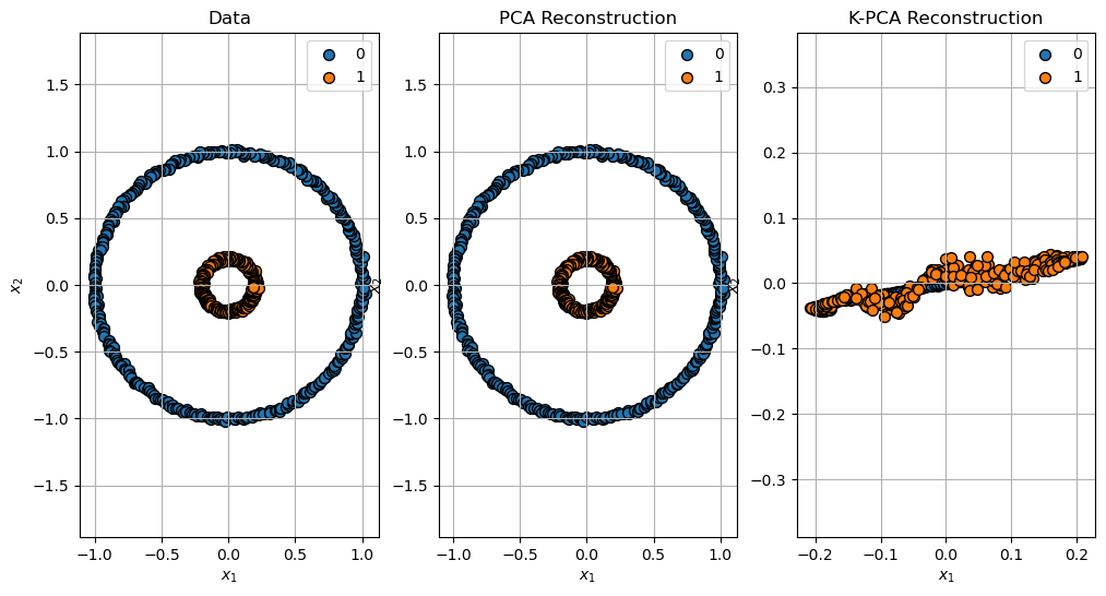
• (?) Explain the reconstruction error of the K-PCA. You may read about the fit_inverse_transform parameter.