
Kernel SVM#
Notebook by:
Royi Avital RoyiAvital@fixelalgorithms.com
Revision History#
Version |
Date |
User |
Content / Changes |
|---|---|---|---|
1.0.000 |
16/03/2024 |
Royi Avital |
First version |
![]()
# Import Packages

# General Tools
import numpy as np
import scipy as sp
import pandas as pd

# Machine Learning
from sklearn.datasets import make_classification
from sklearn.svm import SVC

# Image Processing

# Machine Learning

# Miscellaneous
import math
import os
from platform import python_version
import random
import timeit

# Typing
from typing import Callable, Dict, List, Optional, Set, Tuple, Union

# Visualization
import matplotlib as mpl
import matplotlib.pyplot as plt
import seaborn as sns

# Jupyter
from IPython import get_ipython
from IPython.display import Image
from IPython.display import display
from ipywidgets import Dropdown, FloatSlider, interact, IntSlider, Layout, SelectionSlider
from ipywidgets import interact
Notations#
(?) Question to answer interactively.
(!) Simple task to add code for the notebook.
(@) Optional / Extra self practice.
(#) Note / Useful resource / Food for thought.
Code Notations:
someVar    = 2; #<! Notation for a variable
vVector    = np.random.rand(4) #<! Notation for 1D array
mMatrix    = np.random.rand(4, 3) #<! Notation for 2D array
tTensor    = np.random.rand(4, 3, 2, 3) #<! Notation for nD array (Tensor)
tuTuple    = (1, 2, 3) #<! Notation for a tuple
lList      = [1, 2, 3] #<! Notation for a list
dDict      = {1: 3, 2: 2, 3: 1} #<! Notation for a dictionary
oObj       = MyClass() #<! Notation for an object
dfData     = pd.DataFrame() #<! Notation for a data frame
dsData     = pd.Series() #<! Notation for a series
hObj       = plt.Axes() #<! Notation for an object / handler / function handler
Code Exercise#
Single line fill
vallToFill = ???
Multi Line to Fill (At least one)
# You need to start writing
????
Section to Fill
#===========================Fill This===========================#
# 1. Explanation about what to do.
# !! Remarks to follow / take under consideration.
mX = ???

???
#===============================================================#
# Configuration
# %matplotlib inline

seedNum = 512
np.random.seed(seedNum)
random.seed(seedNum)

# Matplotlib default color palette
lMatPltLibclr = ['#1f77b4', '#ff7f0e', '#2ca02c', '#d62728', '#9467bd', '#8c564b', '#e377c2', '#7f7f7f', '#bcbd22', '#17becf']
# sns.set_theme() #>! Apply SeaBorn theme

runInGoogleColab = 'google.colab' in str(get_ipython())
# Constants

FIG_SIZE_DEF    = (8, 8)
ELM_SIZE_DEF    = 50
CLASS_COLOR     = ('b', 'r')
EDGE_COLOR      = 'k'
MARKER_SIZE_DEF = 10
LINE_WIDTH_DEF  = 2
# Courses Packages
import sys
sys.path.append('../')
sys.path.append('../../')
sys.path.append('../../../')
from utils.DataVisualization import PlotBinaryClassData, PlotDecisionBoundaryClosure
# General Auxiliary Functions

def IsStrFloat(inStr: any) -> bool:
    #Support None input
    if inStr is None:
        return False
    try:
        float(inStr)
        return True
    except ValueError:
        return False
Kernel Trick#
The Kernel Trick is mostly a way to generate features implicitly in a way which is compute efficient.
While it is mostly used in the context of Support Vector Machine (SVM) it is useful in many other algorithms as well.
# Parameters

# Data Generation
numSamples      = 400
numFeatures     = 2 #<! Number of total features
numInformative  = 2 #<! Number of informative features
numRedundant    = 0 #<! Number of redundant features
numRepeated     = 0 #<! Number of repeated features
numClasses      = 2 #<! Number of classes
flipRatio       = 0.05 #<! Number of random swaps

# Data Visualization
numGridPts = 500
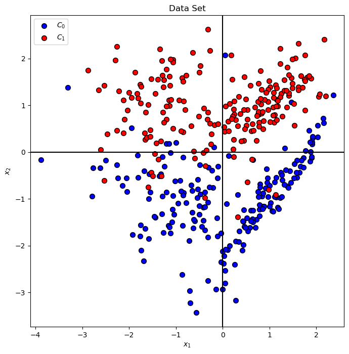
Generate / Load Data#
The data will be generated using SciKit Learn’s make_classification() function.
# Generate Data

mX, vY = make_classification(n_samples = numSamples, n_features = numFeatures, n_informative = numInformative,
                             n_redundant = numRedundant, n_repeated = numRepeated, n_classes = numClasses, flip_y = flipRatio)


# Decision Boundary Plotter
PlotDecisionBoundary = PlotDecisionBoundaryClosure(numGridPts, mX[:, 0].min(), mX[:, 0].max(), mX[:, 1].min(), mX[:, 1].max())

print(f'The features data shape: {mX.shape}')
print(f'The labels data shape: {vY.shape}')
print(f'The unique values of the labels: {np.unique(vY)}')
The features data shape: (400, 2)
The labels data shape: (400,)
The unique values of the labels: [0 1]
Plot Data#
# Plot the Data

hA = PlotBinaryClassData(mX, vY, axisTitle = 'Data Set')
hA.set_xlabel('${x}_{1}$')
hA.set_ylabel('${x}_{2}$')

plt.show()
Train a Kernel SVM Classifier#
The SciKit Learn’s Kernel SVM classifier has 4 kernel options: linear, poly, rbf, sigmoid and manual.
The 2 most used are:
(#) The most commonly used kernel is the RBF kernel.
It can be shown that it is equivalent of potentially infinite polynomial degree where the actual degree can be set using the \(\sigma\) parameter.(#) In case the features are well engineered one can try well tuned linear model. Preferably using
LinearSVCwhich is more efficient with large dataset.
# Kernel SVM Plotting Function

def PlotKernelSvm( C: float, kernelType: str, polyDeg: int, γ: float, mX: np.ndarray, vY: np.ndarray ) -> None:
    if IsStrFloat(γ):
        γ = float(γ)
    # Train the classifier
    oSvmCls = SVC(C = C, kernel = kernelType, degree = polyDeg, gamma = γ).fit(mX, vY) #<! Training on the data, coef0 for bias
    clsScore = oSvmCls.score(mX, vY)

    hF, hA = plt.subplots(figsize = FIG_SIZE_DEF)
    hA = PlotDecisionBoundary(oSvmCls.predict, hA = hA)
    hA = PlotBinaryClassData(mX, vY, hA = hA, axisTitle = f'Classifier Decision Boundary, Accuracy = {clsScore:0.2%}')

    hA.set_xlabel('${x}_{1}$')
    hA.set_ylabel('${x}_{2}$')
# LAmbda Function for Kernel SVM Plot
hPlotKernelSvm = lambda C, kernelType, polyDeg, γ: PlotKernelSvm(C, kernelType, polyDeg, γ, mX, vY)
# Display the Geometry of the Classifier
# Be carful with the degree of the `poly` kernel.

cSlider             = FloatSlider(min = 0.05, max = 3.00, step = 0.05, value = 1.00, layout = Layout(width = '30%'))
kernelTypeDropdown  = Dropdown(options = ['linear', 'poly', 'rbf', 'sigmoid'], value = 'linear', description = 'Kernel Type')
polyDegSlider       = IntSlider(min = 1, max = 10, step = 1, value = 3, layout = Layout(width = '30%'))
γDropdown           = Dropdown(options = ['scale', 'auto', '0.01', '0.05', '0.1', '0.3', '0.5', '0.75', '1.00', '1.50', '2.00', '100.00'], value = 'scale', description = 'Parameter γ')
interact(hPlotKernelSvm, C = cSlider, kernelType = kernelTypeDropdown, polyDeg = polyDegSlider, γ = γDropdown)

plt.show()