K-Means

K-Means#

Notebook by:

Royi Avital RoyiAvital@fixelalgorithms.com

Revision History#

Version	Date	User	Content / Changes
1.0.000	11/04/2024	Royi Avital	First version

# Import Packages

# General Tools
import numpy as np
import scipy as sp
import pandas as pd

# Machine Learning
from sklearn.cluster import KMeans
from sklearn.datasets import make_blobs

# Miscellaneous
import math
import os
from platform import python_version
import random
import timeit

# Typing
from typing import Callable, Dict, List, Optional, Self, Set, Tuple, Union

# Visualization
import matplotlib as mpl
import matplotlib.pyplot as plt
import seaborn as sns

# Jupyter
from IPython import get_ipython
from IPython.display import Image
from IPython.display import display
from ipywidgets import Dropdown, FloatSlider, interact, IntSlider, Layout, SelectionSlider
from ipywidgets import interact

Notations#

(?) Question to answer interactively.
(!) Simple task to add code for the notebook.
(@) Optional / Extra self practice.
(#) Note / Useful resource / Food for thought.

Code Notations:

someVar    = 2; #<! Notation for a variable
vVector    = np.random.rand(4) #<! Notation for 1D array
mMatrix    = np.random.rand(4, 3) #<! Notation for 2D array
tTensor    = np.random.rand(4, 3, 2, 3) #<! Notation for nD array (Tensor)
tuTuple    = (1, 2, 3) #<! Notation for a tuple
lList      = [1, 2, 3] #<! Notation for a list
dDict      = {1: 3, 2: 2, 3: 1} #<! Notation for a dictionary
oObj       = MyClass() #<! Notation for an object
dfData     = pd.DataFrame() #<! Notation for a data frame
dsData     = pd.Series() #<! Notation for a series
hObj       = plt.Axes() #<! Notation for an object / handler / function handler

Code Exercise#

Single line fill

vallToFill = ???

Multi Line to Fill (At least one)

# You need to start writing
????

Section to Fill

#===========================Fill This===========================#
# 1. Explanation about what to do.
# !! Remarks to follow / take under consideration.
mX = ???

???
#===============================================================#

# Configuration
# %matplotlib inline

seedNum = 512
np.random.seed(seedNum)
random.seed(seedNum)

# Matplotlib default color palette
lMatPltLibclr = ['#1f77b4', '#ff7f0e', '#2ca02c', '#d62728', '#9467bd', '#8c564b', '#e377c2', '#7f7f7f', '#bcbd22', '#17becf']
# sns.set_theme() #>! Apply SeaBorn theme

runInGoogleColab = 'google.colab' in str(get_ipython())

# Constants

FIG_SIZE_DEF    = (8, 8)
ELM_SIZE_DEF    = 50
CLASS_COLOR     = ('b', 'r')
EDGE_COLOR      = 'k'
MARKER_SIZE_DEF = 10
LINE_WIDTH_DEF  = 2

# Courses Packages
import sys
sys.path.append('../')
sys.path.append('../../')
sys.path.append('../../../')
from utils.DataVisualization import PlotScatterData

# General Auxiliary Functions

def PlotKMeans( mX: np.ndarray, numClusters: int, numIter: int, initMethod: str = 'random', hA: Optional[plt.Axes] = None, figSize: Tuple[int, int] = FIG_SIZE_DEF, markerSize: int = MARKER_SIZE_DEF ):

    if hA is None:
        hF, hA = plt.subplots(figsize = figSize)
    else:
        hF = hA.get_figure()

    oKMeans = KMeans(n_clusters = numClusters, init = initMethod, n_init = 1, max_iter = numIter, random_state = 0).fit(mX)

    vIdx    = oKMeans.predict(mX)
    mMu     = oKMeans.cluster_centers_
    vor     = sp.spatial.Voronoi(mMu)

    sp.spatial.voronoi_plot_2d(vor, ax = hA, show_points = False, line_width = 2, show_vertices = False)
    hA.scatter(mX[:, 0], mX[:, 1], s = ELM_SIZE_DEF, c = vIdx, edgecolor = EDGE_COLOR)
    hA.plot(mMu[:,0], mMu[:, 1], '.r', markersize = 20)
    hA.axis('equal')
    hA.axis([-12, 8, -12, 8])
    hA.set_xlabel('${{x}}_{{1}}$')
    hA.set_ylabel('${{x}}_{{2}}$')
    hA.set_title(f'K-Means Clustering, Inertia = {oKMeans.inertia_}')

    return hA

Clustering by K-Means#

This notebook demonstrates the use the K-Means for clustering.

# Parameters

# Data Generation
numSamplesCluster   = 150
noiseStd            = 0.1

# Model

# Data Visualization

Generate / Load Data#

Isotropic data clusters.

# Generate Data

mMu = np.array([[4,   4],
                [-3, -3],
                [-2, -8],
                [-8, -2]])

numClusters = mMu.shape[0]
# Generating samples by *Isotropic Gaussian**
mX = np.concatenate([np.random.randn(numSamplesCluster, 2) + vMu for vMu in mMu])
vL = np.repeat(range(numClusters), numSamplesCluster)
numSamples  = mX.shape[0]


print(f'The features data shape: {mX.shape}')

The features data shape: (600, 2)

(?) Where are the labels in this case?

Plot Data#

# Plot the Data

hF, hA = plt.subplots(figsize = (12, 8))

hA = PlotScatterData(mX, vL, hA = hA)

plt.show()

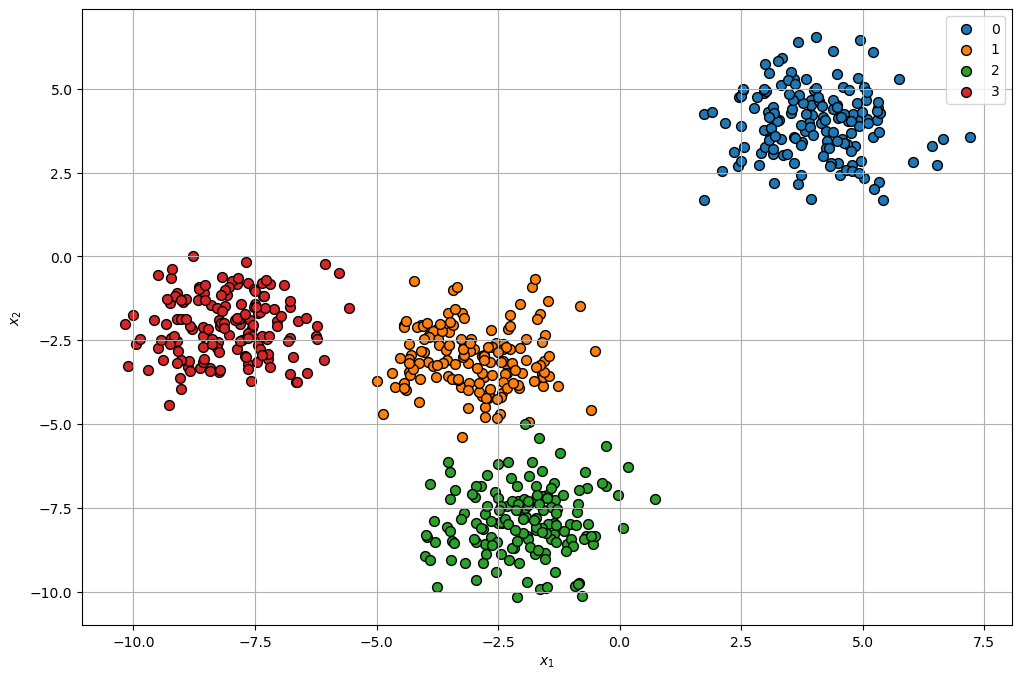
../../../../_images/f53c211c7b849c0249457f61cb09c850e7fc576de2a7af582224b9aa0f4d295d.png

(?) Are there points which are confusing in their labeling?

Cluster Data by K-Means#

Step I:
Assume fixed centroids $\left\{ \boldsymbol{\mu}_{k}\right\} $, find the optimal clusters $\left\{ \mathcal{D}_{k}\right\} $:
$$\arg\min_{\left\{ \mathcal{D}_{k}\right\} }\sum_{k = 1}^{K}\sum_{\boldsymbol{x}_{i}\in\mathcal{D}_{k}}\left\Vert \boldsymbol{x}_{i}-\boldsymbol{\mu}_{k}\right\Vert _{2}^{2}$$\implies \boldsymbol{x}_{i}\in\mathcal{D}_{s\left(\boldsymbol{x}_{i}\right)} \; \text{where} \; s\left(\boldsymbol{x}_{i}\right)=\arg\min_{k}\left\Vert \boldsymbol{x}_{i}-\boldsymbol{\mu}_{k}\right\Vert _{2}^{2}$$
Step II:
Assume fixed clusters $\left\{ \mathcal{D}_{k}\right\} $, find the optimal centroids $\left\{ \boldsymbol{\mu}_{k}\right\} $: $$\arg\min_{\left\{ \boldsymbol{\mu}_{k}\right\} }\sum_{k=1}^{K}\sum_{\boldsymbol{x}_{i}\in\mathcal{D}_{k}}\left\Vert \boldsymbol{x}_{i}-\boldsymbol{\mu}_{k}\right\Vert _{2}^{2}$$\implies\boldsymbol{\mu}_{k}=\frac{1}{\left|\mathcal{D}_{k}\right|}\sum_{\boldsymbol{x}_{i}\in\mathcal{D}_{k}}\boldsymbol{x}_{i}$$
Step III:
Check for convergence (Change in assignments / location of the center). If not, go to Step I.

(#) The K-Means is implemented in KMeans.
(#) Some implementations of the algorithm supports different metrics.

(?) Think of the convergence check options. Think of the cases of large data set vs. small data set.
(?) What does the predict() method in KMeans do?

# Plotting Wrapper

hPlotKMeans = lambda numClusters, numIter, initMethod: PlotKMeans(mX, numClusters = numClusters, numIter = numIter, initMethod = initMethod, figSize = (8, 8))

# Interactive Visualization


numClustersSlider = IntSlider(min = 3, max = 10, step = 1, value = 3, layout = Layout(width = '30%'))
numIterSlider = IntSlider(min = 1, max = 20, step = 1, value = 1, layout = Layout(width = '30%'))
initMethodDropdown = Dropdown(description = 'Initialization Method', options = [('Random', 'random'), ('K-Means++', 'k-means++')], value = 'random')
interact(hPlotKMeans, numClusters = numClustersSlider, numIter = numIterSlider, initMethod = initMethodDropdown)

plt.show()

Assumptions by K-Means Model#

The K-Means has few built in assumptions.
This sections illustrates the cases the assumptions are invalid.

# From SciKit Learn

plt.figure(figsize = (12, 12))

n_samples = 1500
random_state = 170
X, y = make_blobs(n_samples=n_samples, random_state=random_state)

# Incorrect number of clusters
y_pred = KMeans(n_clusters=2, n_init='auto', random_state=random_state).fit_predict(X)

plt.subplot(221)
plt.scatter(X[:, 0], X[:, 1], c=y_pred)
plt.title("Incorrect Number of Blobs")

# Anisotropic distributed data
transformation = [[0.60834549, -0.63667341], [-0.40887718, 0.85253229]]
X_aniso = np.dot(X, transformation)
y_pred = KMeans(n_clusters=3, n_init='auto', random_state=random_state).fit_predict(X_aniso)

plt.subplot(222)
plt.scatter(X_aniso[:, 0], X_aniso[:, 1], c=y_pred)
plt.title("Anisotropic Distributed Blobs")

# Different variance
X_varied, y_varied = make_blobs(n_samples=n_samples, cluster_std=[1.0, 2.5, 0.5], random_state=random_state)
y_pred = KMeans(n_clusters=3, n_init='auto', random_state=random_state).fit_predict(X_varied)

plt.subplot(223)
plt.scatter(X_varied[:, 0], X_varied[:, 1], c=y_pred)
plt.title("Unequal Variance")

# Unevenly sized blobs
X_filtered = np.vstack((X[y == 0][:500], X[y == 1][:100], X[y == 2][:10]))
y_pred = KMeans(n_clusters=3, n_init='auto', random_state=random_state).fit_predict(X_filtered)

plt.subplot(224)
plt.scatter(X_filtered[:, 0], X_filtered[:, 1], c=y_pred)
plt.title("Unevenly Sized Blobs")

plt.show()

Running cells with 'base' requires the ipykernel package.

Run the following command to install 'ipykernel' into the Python environment. 

Command: 'conda install -n base ipykernel --update-deps --force-reinstall'