
Kernel Regression#
Notebook by:
Royi Avital RoyiAvital@fixelalgorithms.com
Revision History#
Version |
Date |
User |
Content / Changes |
|---|---|---|---|
1.0.000 |
01/04/2024 |
Royi Avital |
First version |
![]()
# Import Packages

# General Tools
import numpy as np
import scipy as sp
import pandas as pd

# Machine Learning
from sklearn.linear_model import HuberRegressor, LinearRegression ,RANSACRegressor

# Miscellaneous
import math
import os
from platform import python_version
import random
import timeit

# Typing
from typing import Callable, Dict, List, Optional, Self, Set, Tuple, Union

# Visualization
import matplotlib as mpl
import matplotlib.pyplot as plt
import seaborn as sns

# Jupyter
from IPython import get_ipython
from IPython.display import Image
from IPython.display import display
from ipywidgets import Dropdown, FloatSlider, interact, IntSlider, Layout, SelectionSlider
from ipywidgets import interact
Notations#
(?) Question to answer interactively.
(!) Simple task to add code for the notebook.
(@) Optional / Extra self practice.
(#) Note / Useful resource / Food for thought.
Code Notations:
someVar    = 2; #<! Notation for a variable
vVector    = np.random.rand(4) #<! Notation for 1D array
mMatrix    = np.random.rand(4, 3) #<! Notation for 2D array
tTensor    = np.random.rand(4, 3, 2, 3) #<! Notation for nD array (Tensor)
tuTuple    = (1, 2, 3) #<! Notation for a tuple
lList      = [1, 2, 3] #<! Notation for a list
dDict      = {1: 3, 2: 2, 3: 1} #<! Notation for a dictionary
oObj       = MyClass() #<! Notation for an object
dfData     = pd.DataFrame() #<! Notation for a data frame
dsData     = pd.Series() #<! Notation for a series
hObj       = plt.Axes() #<! Notation for an object / handler / function handler
Code Exercise#
Single line fill
vallToFill = ???
Multi Line to Fill (At least one)
# You need to start writing
????
Section to Fill
#===========================Fill This===========================#
# 1. Explanation about what to do.
# !! Remarks to follow / take under consideration.
mX = ???

???
#===============================================================#
# Configuration
# %matplotlib inline

seedNum = 512
np.random.seed(seedNum)
random.seed(seedNum)

# Matplotlib default color palette
lMatPltLibclr = ['#1f77b4', '#ff7f0e', '#2ca02c', '#d62728', '#9467bd', '#8c564b', '#e377c2', '#7f7f7f', '#bcbd22', '#17becf']
# sns.set_theme() #>! Apply SeaBorn theme

runInGoogleColab = 'google.colab' in str(get_ipython())
# Constants

FIG_SIZE_DEF    = (8, 8)
ELM_SIZE_DEF    = 50
CLASS_COLOR     = ('b', 'r')
EDGE_COLOR      = 'k'
MARKER_SIZE_DEF = 10
LINE_WIDTH_DEF  = 2
# Courses Packages
import sys
sys.path.append('../')
sys.path.append('../../')
sys.path.append('../../../')
from utils.DataVisualization import PlotRegressionData
# General Auxiliary Functions
Kernel Regression#
Kernel Regression is a non parametric regression method.
In this notebook we’ll show the effect of a different kernel and bandwidth on the estimation.
We’ll also show the performance difference between interpolation and extrapolation in the context of Kernel Regression.
(#) The Kernel Regression approach is mostly popular among statisticians in the context of Kernel Density Estimation (KDE). Namely estimating the PDF of a data.
# Parameters

# Data Generation
numSamples  = 200
noiseStd    = 0.01

# Data Visualization
gridNoiseStd = 0.05
numGridPts   = 500
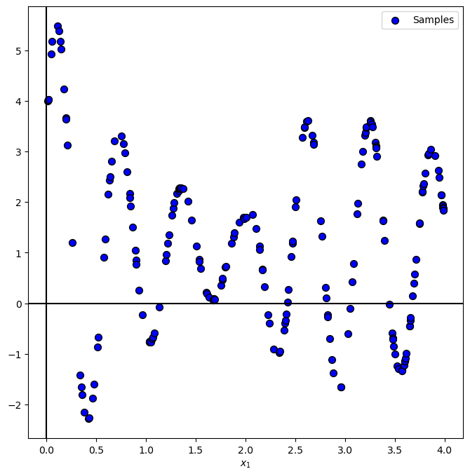
Generate / Load Data#
In the following we’ll generate data according to the following model:
Where
# The Data Generating Function

def f( vX: np.ndarray ):

    return 5 * np.exp(-vX) * np.sin(10 * vX + 0.5) * (1 + 10 * (vX > 2) * (vX - 2)) + 1
# Generate Data

vX = 4 * np.sort(np.random.rand(numSamples))
vY = f(vX) + (noiseStd * np.random.randn(numSamples))

print(f'The features data shape: {vX.shape}')
print(f'The labels data shape: {vY.shape}')
The features data shape: (200,)
The labels data shape: (200,)
Plot Data#
# Plot the Data

PlotRegressionData(vX, vY)

plt.show()
Regression Kernels#
Some of the common kernels are:
Uniform: \(k\left(u\right)=\begin{cases}1 & \left|u\right|\leq\frac{1}{2}\\0 & \text{else}\end{cases}\).
Triangular: \(k\left(u\right)=\begin{cases}1-\left|u\right| & \left|u\right|\leq1\\0 & \text{else}\end{cases}\).
Gaussian: \(k\left(u\right)=e^{-\frac{1}{2}u^{2}}\).
Cosine: \(k\left(u\right)=\begin{cases}1+\cos\left(\pi u\right) & \left|u\right|\leq1\\0 & \text{else}\end{cases}\).
# Defining the Kernels

def UniformKernel( vU: np.ndarray ):
    return 1 * (np.abs(vU) < 0.5)               ### *1 is used to convert the boolean to integer !!! ###

def TriangularKernel( vU: np.ndarray ):
    return (np.abs(vU) < 1) * (1 - np.abs(vU))

def GaussianKernel( vU: np.ndarray ):
    return np.exp(-0.5 * np.square(vU))

def CosineKernel( vU: np.ndarray ):
    return (np.abs(vU) < 1) * (1 + np.cos(np.pi * vU))

lKernels = [('Uniform', UniformKernel), ('Triangular', TriangularKernel), ('Gaussian', GaussianKernel), ('Cosine', CosineKernel)]
(#) In the context of Signal Processing the kernels above are known as a Window Function.
# Plotting the Kernels

hF, hA = plt.subplots(figsize = (10, 6))
vG = np.linspace(-4, 4, numGridPts)

for ii, (kernelLabel, hKernel) in enumerate(lKernels):
    hA.plot(vG, hKernel(vG), lw = 2, label = kernelLabel)

hA.set_xlabel('$x$')
hA.set_ylabel('$y$')
hA.set_title('The Kernels')
hA.legend()
hA.grid()

plt.show()
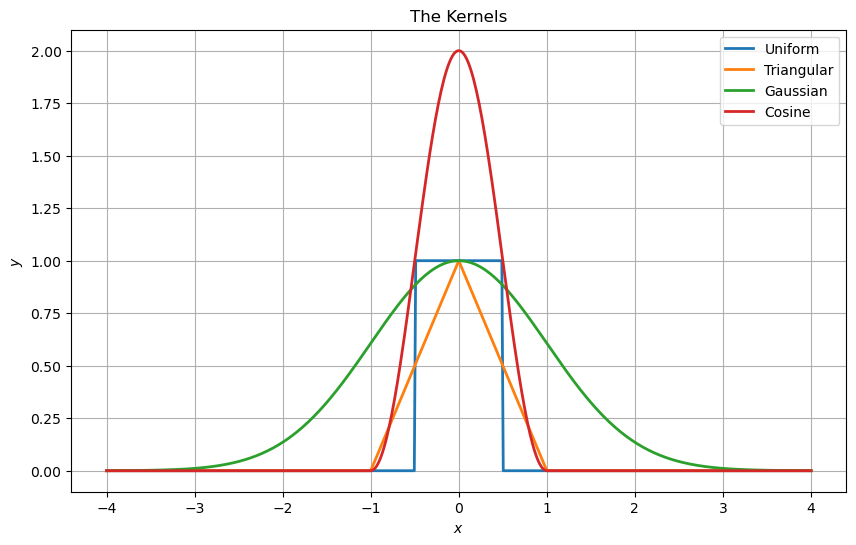
the cos here at the peak is 2 and all other are 1, why?
all function will be normalized - so it is irrelevant.
Kernel Regression#
The kernel regression operation is defined by:
Where \({w}_{x} \left( {x}_{i} \right) = k \left( \frac{ x - x_{i} }{ h } \right)\).
(#) In the context of Signal Processing the operation above is basically a convolution.
a=[1,2,3,4,5,6,7,8,9,10]
a=np.array(a)
print(a)
print(a[:,None])
print(a[None,:])
[ 1  2  3  4  5  6  7  8  9 10]
[[ 1]
 [ 2]
 [ 3]
 [ 4]
 [ 5]
 [ 6]
 [ 7]
 [ 8]
 [ 9]
 [10]]
[[ 1  2  3  4  5  6  7  8  9 10]]
# Applying and Plotting the Kernels

def ApplyKernel( hKernel: Callable[np.ndarray, np.ndarray], paramH: float, vX: np.ndarray, vY: np.ndarray, vG: np.ndarray, zeroThr: float = 1e-9 ) -> np.ndarray:

    mW = hKernel((vG[:, None] - vX[None, :]) / paramH)
    # vYPred = (mW @ vY) / np.sum(mW, axis = 1)
    vK = mW @ vY #<! For numerical stability, removing almost zero values
    vW = np.sum(mW, axis = 1)
    vI = np.abs(vW) < zeroThr #<! Calculate only when there's real data
    vK[vI] = 0
    vW[vI] = 1 #<! Remove cases of dividing by 0
    vYPred = vK / vW

    return vYPred


vG = np.linspace(-0.2, 4.5, 1000, endpoint = True)

def PlotKernelRegression( hKernel: Callable[np.ndarray, np.ndarray], paramH: float, vX: np.ndarray, vY: np.ndarray, vG: np.ndarray, figSize = FIG_SIZE_DEF, hA = None ):

    if hA is None:
        hF, hA = plt.subplots(figsize = figSize)
    else:
        hF = hA.get_figure()

    vYPred = ApplyKernel(hKernel, paramH, vX, vY, vG)

    hA.plot(vG, vYPred, 'b', lw = 2, label = '$\hat{f}(x)$')
    hA.scatter(vX, vY, s = 50, c = 'r', edgecolor = 'k', label = '$y_i = f(x_i) + \epsilon_i$')
    hA.set_title(f'Kernel Regression with h = {paramH}')
    hA.set_xlabel('$x$')
    hA.set_ylabel('$y$')
    hA.grid()
    hA.legend(loc = 'lower right')
hPlotKernelRegression = lambda hK, paramH: PlotKernelRegression(hK, paramH, vX, vY, vG)

hSlider        = FloatSlider(min = 0.001, max = 2.5, step = 0.001, value = 0.01, readout_format = '0.3f', layout = Layout(width = '30%'))
kernelDropdown = Dropdown(options = lKernels, value = GaussianKernel, description = 'Kernel:')
interact(hPlotKernelRegression, hK = kernelDropdown, paramH = hSlider)
plt.show()
(!) Play with the number of samples of the data to see its effect.
(?) What happens outside of the data samples? What does it mean for real world data?
exterpolution is dumping to zero :
