Features Transform case2

Polynomial and Coordinate Change Feature Transform as a Pipeline.

Notebook by:

• Royi Avital RoyiAvital@fixelalgorithms.com

Revision History

Version	Date	User	Content / Changes
1.0.000	16/03/2024	Royi Avital	First version

# Import Packages

# General Tools
import numpy as np
import scipy as sp
import pandas as pd

# Machine Learning
from sklearn.base import TransformerMixin
from sklearn.datasets import make_circles
from sklearn.pipeline import Pipeline
from sklearn.preprocessing import PolynomialFeatures
from sklearn.svm import SVC

# Image Processing

# Machine Learning

# Miscellaneous
import math
import os
from platform import python_version
import random
import timeit

# Typing
from typing import Callable, Dict, List, Optional, Set, Tuple, Union

# Visualization
import matplotlib as mpl
import matplotlib.pyplot as plt
import seaborn as sns

# Jupyter
from IPython import get_ipython
from IPython.display import Image
from IPython.display import display
from ipywidgets import Dropdown, FloatSlider, interact, IntSlider, Layout, SelectionSlider
from ipywidgets import interact

Notations

• (?) Question to answer interactively.

• (!) Simple task to add code for the notebook.

• (@) Optional / Extra self practice.

• (#) Note / Useful resource / Food for thought.

Code Notations:

someVar    = 2; #<! Notation for a variable
vVector    = np.random.rand(4) #<! Notation for 1D array
mMatrix    = np.random.rand(4, 3) #<! Notation for 2D array
tTensor    = np.random.rand(4, 3, 2, 3) #<! Notation for nD array (Tensor)
tuTuple    = (1, 2, 3) #<! Notation for a tuple
lList      = [1, 2, 3] #<! Notation for a list
dDict      = {1: 3, 2: 2, 3: 1} #<! Notation for a dictionary
oObj       = MyClass() #<! Notation for an object
dfData     = pd.DataFrame() #<! Notation for a data frame
dsData     = pd.Series() #<! Notation for a series
hObj       = plt.Axes() #<! Notation for an object / handler / function handler

Code Exercise

• Single line fill

vallToFill = ???

• Multi Line to Fill (At least one)

# You need to start writing
????

• Section to Fill

#===========================Fill This===========================#
# 1. Explanation about what to do.
# !! Remarks to follow / take under consideration.
mX = ???

???
#===============================================================#

# Configuration
# %matplotlib inline

seedNum = 512
np.random.seed(seedNum)
random.seed(seedNum)

# Matplotlib default color palette
lMatPltLibclr = ['#1f77b4', '#ff7f0e', '#2ca02c', '#d62728', '#9467bd', '#8c564b', '#e377c2', '#7f7f7f', '#bcbd22', '#17becf']
# sns.set_theme() #>! Apply SeaBorn theme

runInGoogleColab = 'google.colab' in str(get_ipython())

# Constants

FIG_SIZE_DEF    = (8, 8)
ELM_SIZE_DEF    = 50
CLASS_COLOR     = ('b', 'r')
EDGE_COLOR      = 'k'
MARKER_SIZE_DEF = 10
LINE_WIDTH_DEF  = 2

# Courses Packages
import sys
sys.path.append('../')
sys.path.append('../../')
sys.path.append('../../../')
from utils.DataVisualization import PlotBinaryClassData, PlotDecisionBoundaryClosure

# General Auxiliary Functions

Features Transform

In this exercise we’ll apply a feature transform to solve a classification problem.
We’ll apply 2 different transforms:

1. Polynomial Transform

2. Polar Coordinates.

In the exercise we’ll learn about 2 features of SciKit Learn:

1. Pre Processing Module.

2. Pipelines.

The tasks are:

1. Train a linear SVM classifier on the data to have a base line.

2. Apply polynomial feature transform using PolynomialFeatures.

3. Train a linear SVM classifier on the transformed features.

4. Change coordinates of the original features to Polar Coordinate System.

5. Train a linear SVM classifier on the transformed features.

• (#) See Data Science - List of Feature Engineering Techniques.

• (#) See Data Science - Tools for Feature Engineering.

• (#) See SciKit Learn’s Time Related Feature Engineering.

• (#) FeatureTools is a well known tool for feature generation.

• (#) Some useful tutorials on Feature Engineering are given in: Feature Engine, Feature Engine Examples, Python Feature Engineering Cookbook - Jupyter Notebooks.

# Parameters

# Data Generation
numSamples = 250 #<! Per Quarter

# Pre Processing
polyDeg = 2

# Model
paramC      = 1
kernelType  = 'linear'
lC          = [0.1, 0.25, 0.75, 1, 1.5, 2, 3]

# Data Visualization
numGridPts = 500

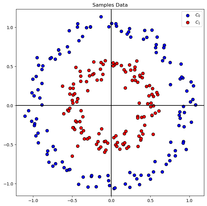
Generate / Load Data

# Generate Data 

mX, vY  = make_circles(n_samples = numSamples, shuffle = True, noise = 0.075, factor = 0.50)

PlotDecisionBoundary = PlotDecisionBoundaryClosure(numGridPts, -1.5, 1.5, -1.5, 1.5)

print(f'The features data shape: {mX.shape}')
print(f'The labels data shape: {vY.shape}')
print(f'The unique values of the labels: {np.unique(vY)}')

The features data shape: (250, 2)
The labels data shape: (250,)
The unique values of the labels: [0 1]

Plot Data

# Plot the Data

hA = PlotBinaryClassData(mX, vY, axisTitle = 'Samples Data')

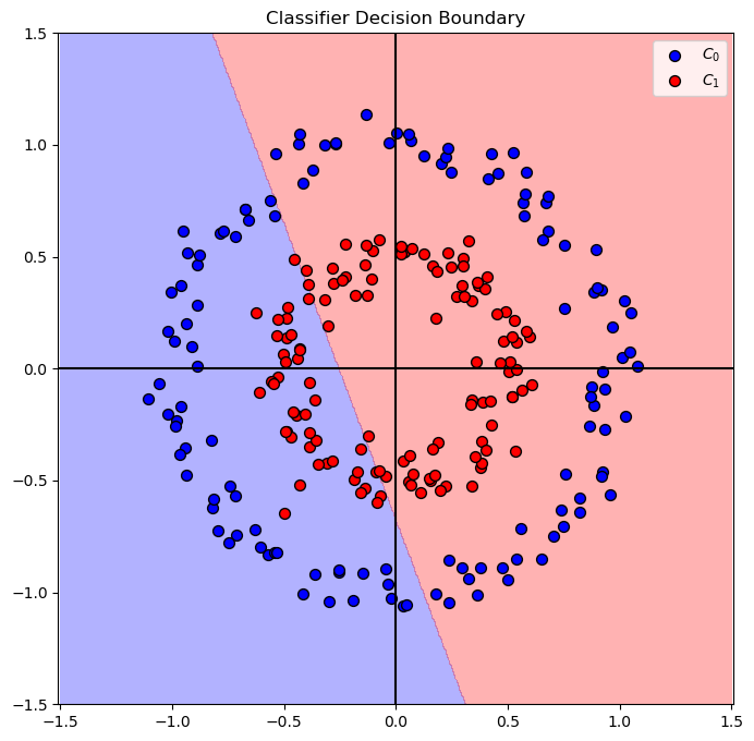
Train a Linear SVM Model

In this section we’ll try optimize the best Linear SVM model for the problem.

• (?) What do you think the decision boundary will be?

# SVM Linear Model
# Optimize the `C` hyper parameter of the linear SVM model.

vAcc = np.zeros(shape = len(lC)) #<! Array of accuracy

#===========================Fill This===========================#
# 1. Iterate over the parameters in `lC`.
# 2. Score each model.
# 3. Extract the best model.

for ii, C in enumerate(lC):
    oLinSvc  = SVC(C = C, kernel = kernelType).fit(mX, vY) #<! Model definition and training
    vAcc[ii] = oLinSvc.score(mX, vY) #<! Accuracy

bestModelIdx    = np.argmax(vAcc)
bestC           = lC[bestModelIdx]

oLinSvc = SVC(C = bestC , kernel = kernelType).fit(mX, vY) #<! Best model

#===============================================================#

print(f'The best model with C = {bestC:0.2f} achieved accuracy of {vAcc[bestModelIdx]:0.2%}')

The best model with C = 0.10 achieved accuracy of 54.80%

# Plot the Decision Boundary

hF, hA = plt.subplots(figsize = FIG_SIZE_DEF)
hA = PlotDecisionBoundary(oLinSvc.predict, hA)
hA = PlotBinaryClassData(mX, vY, hA = hA, axisTitle = 'Classifier Decision Boundary')
plt.show()

Feature Transform

In this section we’ll create a new set of features.
We’ll have 2 types of transformations:

1. Polynomial.

2. Polar Coordinates.

In order to apply the chain of operation: X -> PolyFeatures -> Model we’ll create a SciKit Pipeline using Pipeline.
The concept of a pipeline is creating a SciKit Learn object (With the fit(), predict() approach) which chains multiple objects and allows simpler optimization of the whole process.

Polynomial Features Transform

The features will model a higher degree polynomial base don the 2 given features (Coordinates).

Given the data as:

\[ X = \begin{bmatrix} \boldsymbol{x}_{1} & \boldsymbol{x}_{2} \end{bmatrix} \]

We’ll generate the matrix:

\[ \bar{X} = \begin{bmatrix} \boldsymbol{x}_{1} & \boldsymbol{x}_{2} & \boldsymbol{x}_{1} \otimes \boldsymbol{x}_{1} & \boldsymbol{x}_{2} \otimes \boldsymbol{x}_{2} & \boldsymbol{x}_{1} \otimes \boldsymbol{x}_{2} & \dots \end{bmatrix} \]

Where \(\otimes\) is the Kronecker Product, element wise multiplication.

Basically we create all inter multiplication up to order \(p\) of the data.
This is done using PolynomialFeatures from the preprocessing module of SciKit Learn.

• (?) Given we’re using the SVM model, do we need the term \(\boldsymbol{1}\) in our features? Look at the include_bias parameter in PolynomialFeatures.

• (?) Why is the polyDeg parameter set to 2?

polyDeg

2

# Construct the PolynomialFeatures Object



# Generate a new feature matrix consisting of all polynomial combinations of the features 
# with degree less than or equal to the specified degree. For example, if an input sample 
# is two dimensional and of the form [a, b], the degree-2 polynomial features are 
# [1, a, b, a^2, ab, b^2].


# include_biasbool, default=True
#     If True (default), then include a bias column,
#  the feature in which all polynomial powers are zero 
# (i.e. a column of ones - acts as an intercept term in a linear model).


#===========================Fill This===========================#
# 1. Set the `degree` and pay attention to `include_bias` parameter.
oPolyTrns = PolynomialFeatures(degree = polyDeg, include_bias = False)
#===============================================================#

# Feature Generation
# Generate a set of features by applying the transformations.

#===========================Fill This===========================#
# 1. Read about the fit() and transform() methods of PolynomialFeatures.
 
#  fit(X, y=None)[source]
#    Compute number of output features

#  transform(X)[source]
#   Transform data to polynomial features.

# 2. Use the methods to apply the feature transform.
oPolyTrns = oPolyTrns.fit(mX)
mX1 = oPolyTrns.transform(mX)
#===============================================================#

print(f'shape of the original data: {mX.shape}')
print(f'shape of the transformed data: {mX1.shape}')

shape of the original data: (250, 2)
shape of the transformed data: (250, 5)

# SVM Linear Model
# Apply a linear model on the transformed features.

vAcc = np.zeros(shape = len(lC)) #<! Array of accuracy

#===========================Fill This===========================#
# 1. Iterate over the parameters in `lC`.
# 2. Score each model.
# 3. Extract the best model.
# !! Make sure to use the transformed features.

for ii, C in enumerate(lC):
    oLinSvc  = SVC(C=C , kernel= kernelType).fit(mX1,vY) #<! Model definition and training
    vAcc[ii] = oLinSvc.score(mX1, vY) #<! Accuracy

bestModelIdx    = np.argmax(vAcc)
bestC           = lC[bestModelIdx]

oLinSvc = SVC(C=bestC , kernel= kernelType).fit(mX1,vY) #<! Best model

#===============================================================#

print(f'The best model with C = {bestC:0.2f} achieved accuracy of {vAcc[bestModelIdx]:0.2%}')

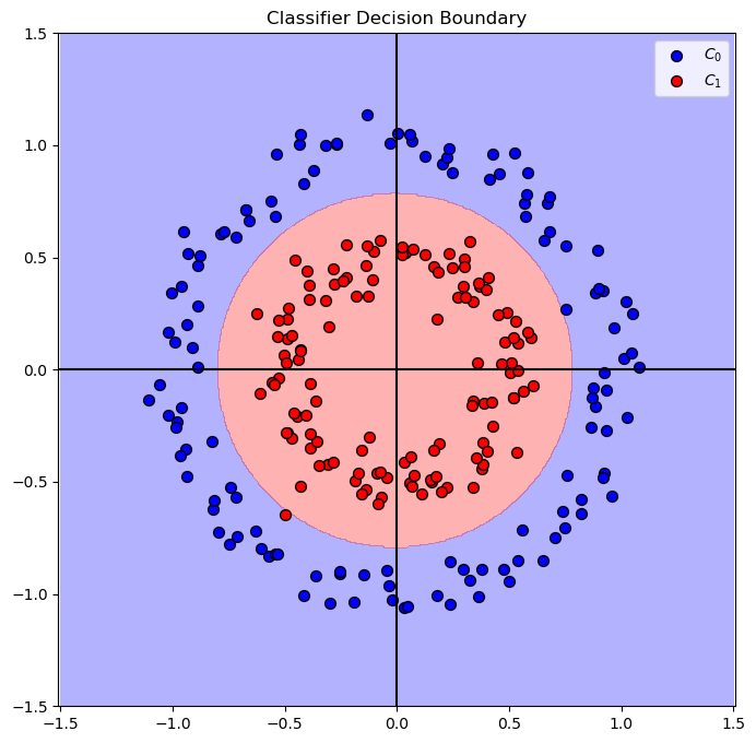
The best model with C = 0.25 achieved accuracy of 99.60%

Decision Boundary

• (?) Can we apply the trained model on the original feature set? Think about dimensions of the data.

In order to plot the decision boundary over the original features we need to have a single object, with the predict() method to apply both the pre processing and the prediction.
This is the basic concept behind a pipeline in SciKit Learn.

• (#) Later on we’ll use this concept for the training step as well.

# Build the Pipeline

#===========================Fill This===========================#
# 1. Construct the pipeline object.
# 2. The 1st step is `Transformer` which applies the polynomial transformation.
# 3. The 2nd step is `Classifier` which applies the classifier.
oModelPipe = Pipeline([('Transformer', oPolyTrns), ('Classifier', oLinSvc)])
#===============================================================#

# Plot the Decision Boundary

hF, hA = plt.subplots(figsize = FIG_SIZE_DEF)
hA = PlotDecisionBoundary(oModelPipe.predict, hA)
hA = PlotBinaryClassData(mX, vY, hA = hA, axisTitle = 'Classifier Decision Boundary')
plt.show()

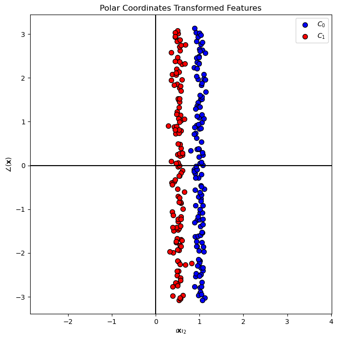
Polar Coordinates

In this section we’ll replace the features with the following model:

\[ \phi \left( {x}_{1}, {x}_{2} \right) \to \left( \sqrt{ {x}_{1}^{2} + {x}_{2}^{2} }, \angle \left( {x}_{1}, {x}_{2} \right) \right) \]

Where \(\angle \left( {x}_{1}, {x}_{2} \right)\) is the angle between the point \(\left( {x}_{1}, {x}_{2} \right)\) to the positive direction of \({x}_{1}\) axis.

• (#) This is an example of a domain knowledge like transformation while the previous case is AutoML case.

Then we’ll show the decision boundary of the best model.

• (?) What do you expect the decision boundary to like in this time?

The tasks:

1. Create a transformer sub class to apply the data transformation.

2. Apply the transform on the data and plot it to verify it.

3. Create a pipeline based on the data using a pre defined parameters for the SVM model.

4. Train the pipeline using fit().

5. Plot the decision boundary.

• (#) Later on we’ll learn how to control the parameters of the steps of a pipeline.

# The PolarCoordinatesTransformer Class
# This is a SciKit Learn transformer sub class.
# This class implements the `fit()`, `transform()` and `fit_transform()` methods.


class PolarCoordinatesTransformer(TransformerMixin):
    def __init__(self):
        pass

    def fit(self, mX, vY = None):
#===========================Fill This===========================#
# This method gets the input features and allocate memory for the transformed features.
# It also keeps, for later validation, the dimensions of the input data.
        numSamples  = mX.shape[0]
        dataDim     = mX.shape[1]
        if dataDim != 2:
            raise ValueError(f'The input data must have exactly 2 columns while it has {dataDim} columns')
        
        mZ = np.empty(shape = (numSamples, 2)) #<! Allocate output

        self.numSamples = numSamples
        self.dataDim    = dataDim
        self.mZ         = mZ

        return self
#===============================================================#
    
    def transform(self, mX):
#===========================Fill This===========================#
# This method applies the actual transform.
# It saves the transformations into `mZ`.
# The 1st column is the magnitude and the 2nd column is the angle.
        if ((mX.shape[0] != self.numSamples) or (mX.shape[1] != self.dataDim)):
            raise ValueError(f'The data to transform has a different dimensions than the data which defined in `fit()`')
        
        self.mZ[:, 0] = np.linalg.norm(mX, axis = 1) #<! Norm
        self.mZ[:, 1] = np.arctan2(mX[:, 1], mX[:, 0]) #<! Angle

        return self.mZ
#===========================Fill This===========================#

    def fit_transform(self, mX, vY = None, **fit_params):
        
        return super().fit_transform(mX, vY, **fit_params)

• (!) The class above calculates \({\left\| \boldsymbol{x} \right\|}_{2}\). Implement \({\left\| \boldsymbol{x} \right\|}_{2}^{2}\) instead and compare results.

• (?) Which of the option would you chose for production?

# Transformer Object

#===========================Fill This===========================#
# 1. Construct the PolarCoordinatesTransformer object.
oPolarTrns = PolarCoordinatesTransformer()
#===============================================================#

# Apply Transformation

#===========================Fill This===========================#
# 1. Generate a set of features with the new feature.
# 2. Use fit_transform() to both fit and apply at once.
mX2 = oPolarTrns.fit_transform(mX)
#===============================================================#

print(f'shape of the original data: {mX.shape}')
print(f'shape of the transformed data: {mX2.shape}')

shape of the original data: (250, 2)
shape of the transformed data: (250, 2)

# Plot the Transformed Features
hF, hA = plt.subplots(figsize = FIG_SIZE_DEF)
hA = PlotBinaryClassData(mX2, vY, hA = hA, axisTitle = 'Polar Coordinates Transformed Features')
hA.set_xlabel(r'${\left\Vert \bf{x} \right\Vert}_{2}$')
hA.set_ylabel(r'$ \angle \left( \bf{x} \right) $')

plt.show()

# SVM Linear Model - On the Transformed Data

vAcc = np.zeros(shape = len(lC))

for ii, C in enumerate(lC):
    oLinSvc  = SVC(C = C, kernel = kernelType).fit(mX2, vY)
    vAcc[ii] = oLinSvc.score(mX2, vY)

bestModelIdx    = np.argmax(vAcc)
bestC           = lC[bestModelIdx]

oLinSvc = SVC(C = bestC, kernel = kernelType).fit(mX2, vY)

print(f'The best model with C = {bestC:0.2f} achieved accuracy of {vAcc[bestModelIdx]:0.2%}')

The best model with C = 0.10 achieved accuracy of 99.60%

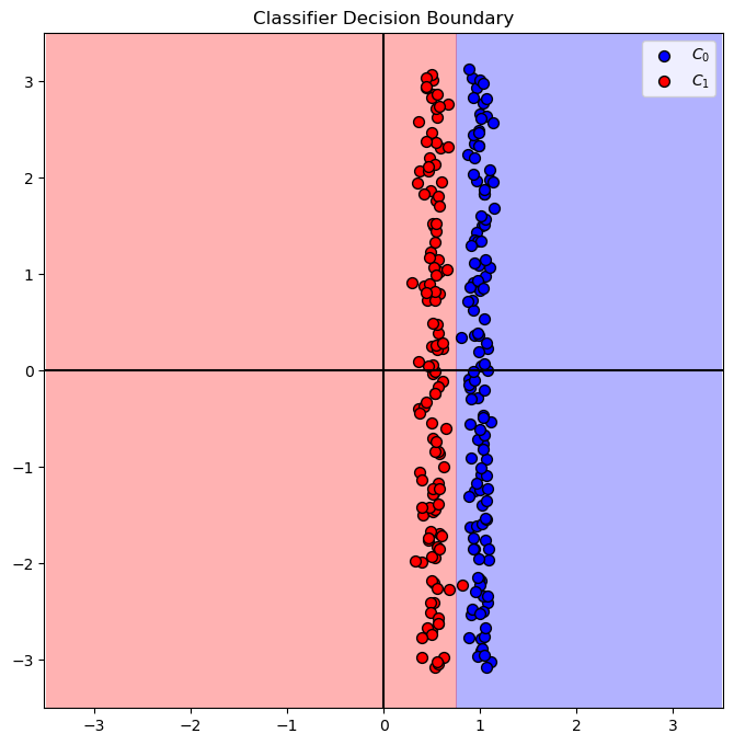
# Plot the Decision Boundary

PlotDecisionBoundary = PlotDecisionBoundaryClosure(numGridPts, 0, 2, -3.5, 3.5)

hF, hA = plt.subplots(figsize = FIG_SIZE_DEF)
hA = PlotDecisionBoundary(oLinSvc.predict, hA)
hA = PlotBinaryClassData(mX2, vY, hA = hA, axisTitle = 'Classifier Decision Boundary')
plt.show()

# Build the Pipeline

oPolarTrns = oPolarTrns.fit(np.zeros(shape = (numGridPts * numGridPts, 2))) #<! Fitting to the grid of the plot

#===========================Fill This===========================#
# 1. Construct the pipeline object.
# 2. The 1st step is `Transformer` which applies the polynomial transformation.
# 3. The 2nd step is `Classifier` which applies the classifier.
oModelPipe = Pipeline([('Transformer', oPolarTrns), ('Classifier', oLinSvc)])
#===============================================================#

# Plot the Decision Boundary

PlotDecisionBoundary = PlotDecisionBoundaryClosure(numGridPts, -1.5, 1.5, -1.5, 1.5)

hF, hA = plt.subplots(figsize = FIG_SIZE_DEF)
hA = PlotDecisionBoundary(oModelPipe.predict, hA)
hA = PlotBinaryClassData(mX, vY, hA = hA, axisTitle = 'Classifier Decision Boundary')
plt.show()

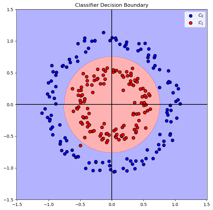
• (?) Do we need both features?

• (?) How would you solve the case above?

• (!) Try with random seed seedNum = 512. Explain results.