Features Transform case1

Notebook by:

• Royi Avital RoyiAvital@fixelalgorithms.com

Revision History

Version	Date	User	Content / Changes
1.0.000	16/03/2024	Royi Avital	First version

# Import Packages

# General Tools
import numpy as np
import scipy as sp
import pandas as pd

# Machine Learning
from sklearn.svm import SVC

# Image Processing

# Machine Learning

# Miscellaneous
import math
import os
from platform import python_version
import random
import timeit

# Typing
from typing import Callable, Dict, List, Optional, Set, Tuple, Union

# Visualization
import matplotlib as mpl
import matplotlib.pyplot as plt
import seaborn as sns

# Jupyter
from IPython import get_ipython
from IPython.display import Image
from IPython.display import display
from ipywidgets import Dropdown, FloatSlider, interact, IntSlider, Layout, SelectionSlider
from ipywidgets import interact

Notations

• (?) Question to answer interactively.

• (!) Simple task to add code for the notebook.

• (@) Optional / Extra self practice.

• (#) Note / Useful resource / Food for thought.

Code Notations:

someVar    = 2; #<! Notation for a variable
vVector    = np.random.rand(4) #<! Notation for 1D array
mMatrix    = np.random.rand(4, 3) #<! Notation for 2D array
tTensor    = np.random.rand(4, 3, 2, 3) #<! Notation for nD array (Tensor)
tuTuple    = (1, 2, 3) #<! Notation for a tuple
lList      = [1, 2, 3] #<! Notation for a list
dDict      = {1: 3, 2: 2, 3: 1} #<! Notation for a dictionary
oObj       = MyClass() #<! Notation for an object
dfData     = pd.DataFrame() #<! Notation for a data frame
dsData     = pd.Series() #<! Notation for a series
hObj       = plt.Axes() #<! Notation for an object / handler / function handler

Code Exercise

• Single line fill

vallToFill = ???

• Multi Line to Fill (At least one)

# You need to start writing
????

• Section to Fill

#===========================Fill This===========================#
# 1. Explanation about what to do.
# !! Remarks to follow / take under consideration.
mX = ???

???
#===============================================================#

# Configuration
# %matplotlib inline

seedNum = 512
np.random.seed(seedNum)
random.seed(seedNum)

# Matplotlib default color palette
lMatPltLibclr = ['#1f77b4', '#ff7f0e', '#2ca02c', '#d62728', '#9467bd', '#8c564b', '#e377c2', '#7f7f7f', '#bcbd22', '#17becf']
# sns.set_theme() #>! Apply SeaBorn theme

runInGoogleColab = 'google.colab' in str(get_ipython())

# Constants

FIG_SIZE_DEF    = (8, 8)
ELM_SIZE_DEF    = 50
CLASS_COLOR     = ('b', 'r')
EDGE_COLOR      = 'k'
MARKER_SIZE_DEF = 10
LINE_WIDTH_DEF  = 2

# Courses Packages
import sys
sys.path.append('../')
sys.path.append('../../')
sys.path.append('../../../')
from utils.DataVisualization import PlotBinaryClassData, PlotDecisionBoundaryClosure

# General Auxiliary Functions

Feature Engineering

Feature Engineering is the art of classic machine learning.
Given that most models are known to all, the feature engineering step is the one most important along with the hyper parameter optimization.

It mostly composed of:

• Feature Transform / Extraction
  Applying operators to generate additional features out of the given features.
  The operations can be: Polynomial, Statistical, Normalization, Change of Coordinates, etc…

• Dimensionality Reduction
  A specific case of transform which reduce the number of features to maximize the inner structure of the data.

• Feature Selection
  A specific case of dimensionality reduction where only a sub set of the features are used.
  They are selected by statistical tests or closed loop evaluation.

Some also include Pre Process steps as handling missing data and outlier rejection as part of the feature engineering step.

The motivation of a specific processing is a result of:

1. Domain Knowledge
   The knowledge about the origins and the domain of data.
   For instance, if one works on RF Data, analyzing the Fourier Domain features is a domain knowledge.

2. AutoML
   Building a loop which evaluates the hyper parameters of the feature engineering steps to maximize the score.
   Commonly some automated feature generators are incorporated into the loop.

Some domains have their own specific approaches. For instance, in Time Series Forecasting there are methods which assists with dealing with the periodicity of the data.

• (#) See Data Science - List of Feature Engineering Techniques.

• (#) See Data Science - Tools for Feature Engineering.

• (#) See SciKit Learn’s Time Related Feature Engineering.

• (#) FeatureTools is a well known tool for feature generation.

Kernel SVM by Feature Transform

In this notebook we’ll imitate the effect of the Kernel Trick using features transform.
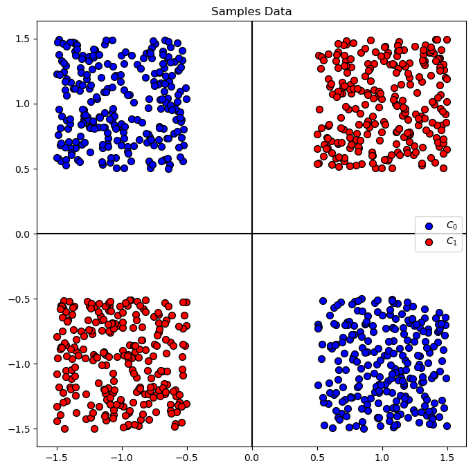
We’ll use a XOR Data Set, where data are located in the 4 quadrants of the \(\mathbb{R}^{2}\) space.

• (#) Some useful tutorials on Feature Engineering are given in: Feature Engine, Feature Engine Examples, Python Feature Engineering Cookbook - Jupyter Notebooks.

# Parameters

# Data Generation
numSamples = 250 #<! Per Quarter

# Model
paramC      = 1
kernelType  = 'linear'
lC          = [0.1, 0.25, 0.75, 1, 1.5, 2, 3]

# Data Visualization
numGridPts = 500

Generate / Load Data

# Generate Data 

mX1  = np.random.rand(numSamples, 2) - 0.5 + np.array([ 1,  1]).T
mX2  = np.random.rand(numSamples, 2) - 0.5 + np.array([-1, -1]).T
mX3  = np.random.rand(numSamples, 2) - 0.5 + np.array([-1,  1]).T
mX4  = np.random.rand(numSamples, 2) - 0.5 + np.array([ 1, -1]).T

mX = np.concatenate((mX1, mX2, mX3, mX4), axis = 0)
vY = np.concatenate((np.full(2 * numSamples, 1), np.full(2 * numSamples, 0)))


PlotDecisionBoundary = PlotDecisionBoundaryClosure(numGridPts, -1.5, 1.5, -1.5, 1.5)

print(f'The features data shape: {mX.shape}')
print(f'The labels data shape: {vY.shape}')
print(f'The unique values of the labels: {np.unique(vY)}')

The features data shape: (1000, 2)
The labels data shape: (1000,)
The unique values of the labels: [0 1]

Plot Data

# Plot the Data

hA = PlotBinaryClassData(mX, vY, axisTitle = 'Samples Data')

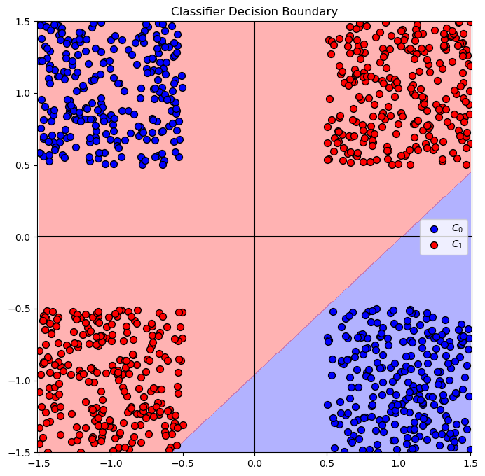
Train a Linear SVM Model

• (?) Given the data, what do you expect the best accuracy will be?

# SVM Linear Model

vAcc = np.zeros(shape = len(lC))

for ii, C in enumerate(lC):
    oLinSvc  = SVC(C = C, kernel = kernelType).fit(mX, vY)
    vAcc[ii] = oLinSvc.score(mX, vY)

bestModelIdx    = np.argmax(vAcc)
bestC           = lC[bestModelIdx]

oLinSvc = SVC(C = bestC, kernel = kernelType).fit(mX, vY)

print(f'The best model with C = {bestC:0.2f} achieved accuracy of {vAcc[bestModelIdx]:0.2%}')

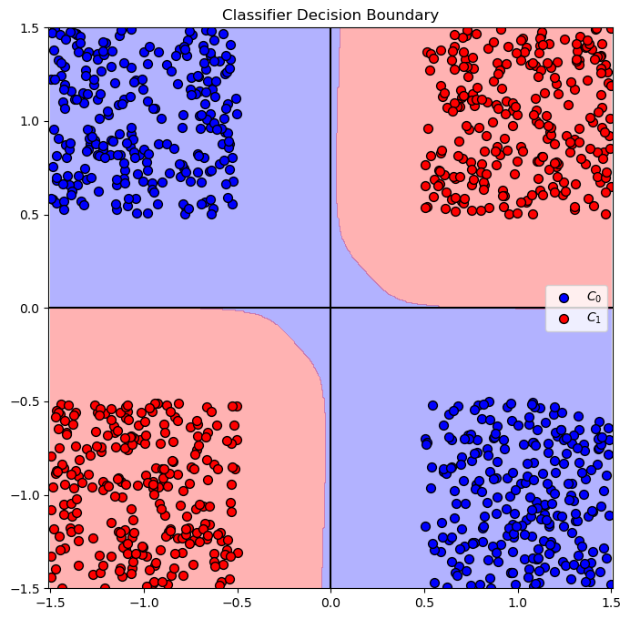
The best model with C = 1.00 achieved accuracy of 75.00%

why only 75? svm take to min the dist

dist is not a loss !!!!

# Plot the Decision Boundary

hF, hA = plt.subplots(figsize = FIG_SIZE_DEF)
hA = PlotDecisionBoundary(oLinSvc.predict, hA)
hA = PlotBinaryClassData(mX, vY, hA = hA, axisTitle = 'Classifier Decision Boundary')
plt.show()

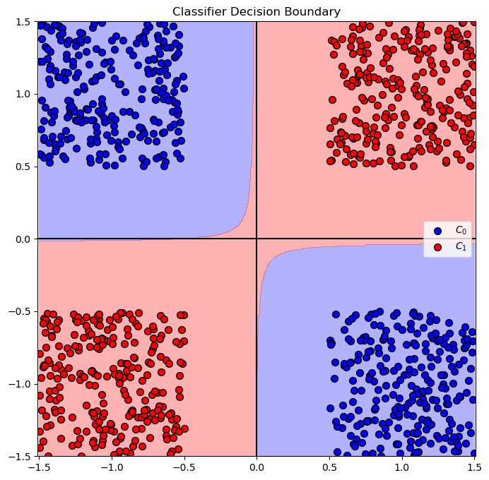
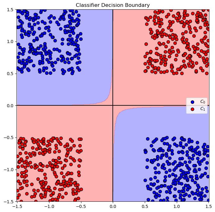
Feature Transform

In this section we’ll a new feature: \({x}_{3} = {x}_{1} \cdot {x}_{2}\).

# Generate a set of features with the new feature
mXX = np.column_stack((mX, mX[:, 0] * mX[:, 1]))
print(f'mx shape = {mX.shape}')
print(f'mxx shape = {mXX.shape}')       ### increase the number of features !!!!

mx shape = (1000, 2)
mxx shape = (1000, 3)

Solution by Linear SVM Classifier

In this section we’ll try optimize the best Linear SVM model for the problem.
Yet, we’ll train it on the features with the additional transformed one.

Then we’ll show the decision boundary of the best model.

• (?) What do you expect the decision boundary to look like this time?

# SVM Linear Model

vAcc = np.zeros(shape = len(lC))

for ii, C in enumerate(lC):
    oLinSvc  = SVC(C = C, kernel = kernelType).fit(mXX, vY) #<! Pay attention we train on `mXX`
    vAcc[ii] = oLinSvc.score(mXX, vY)

bestModelIdx    = np.argmax(vAcc)
bestC           = lC[bestModelIdx]

oLinSvc = SVC(C = bestC, kernel = kernelType).fit(mXX, vY)

print(f'The best model with C = {bestC:0.2f} achieved accuracy of {vAcc[bestModelIdx]:0.2%}')

The best model with C = 0.10 achieved accuracy of 100.00%

• (?) Why was the above C gave the best results?

• (?) What’s the accuracy of all other models?

lC

[0.1, 0.25, 0.75, 1, 1.5, 2, 3]

!!! the C is not important here because the data is linearly separable !!!!

# Plot the Decision Boundary

hPredict = lambda mX: oLinSvc.predict(np.column_stack((mX, mX[:, 0] * mX[:, 1])))

hF, hA = plt.subplots(figsize = FIG_SIZE_DEF)
hA = PlotDecisionBoundary(hPredict, hA)
hA = PlotBinaryClassData(mX, vY, hA = hA, axisTitle = 'Classifier Decision Boundary')
plt.show()

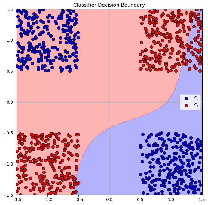
Solution by Kernel SVM - Polynomial

In this section we’ll apply a Kernel SVM with Polynomial kernel.

• (?) What feature transform is needed for this model?

• (?) What’s the minimum degree of the polynomial to solve this problem?

# SVM Polynomial Model

pDegree     = 4
kernelType  = 'poly'

vAcc = np.zeros(shape = len(lC))

for ii, C in enumerate(lC):
    oSvc     = SVC(C = C, kernel = kernelType, degree = pDegree).fit(mX, vY)
    vAcc[ii] = oSvc.score(mX, vY)

bestModelIdx    = np.argmax(vAcc)
bestC           = lC[bestModelIdx]

oSvc = SVC(C = bestC, kernel = kernelType, degree = pDegree).fit(mX, vY)

print(f'The best model with C = {bestC:0.2f} achieved accuracy of {vAcc[bestModelIdx]:0.2%}')

The best model with C = 0.10 achieved accuracy of 100.00%

# Plot the Decision Boundary

hF, hA = plt.subplots(figsize = FIG_SIZE_DEF)
hA = PlotDecisionBoundary(oSvc.predict, hA)
hA = PlotBinaryClassData(mX, vY, hA = hA, axisTitle = 'Classifier Decision Boundary')
plt.show()

• (@) Do the above with the rbf and sigmoid kernels.

• (!) Run the above with the kernel poly and set degree to 100. What happened?

• (?) How will the complexity of the calculation grow with the polynomial degree?

• (#) The issues above are the motivation for the Kernel Trick.

Test with RBF kernel

kernelType  = 'rbf'

vAcc = np.zeros(shape = len(lC))

for ii, C in enumerate(lC):
    oSvc     = SVC(C = C, kernel = kernelType).fit(mX, vY)
    vAcc[ii] = oSvc.score(mX, vY)

bestModelIdx    = np.argmax(vAcc)
bestC           = lC[bestModelIdx]

oSvc = SVC(C = bestC, kernel = kernelType, degree = pDegree).fit(mX, vY)

print(f'The best model with C = {bestC:0.2f} achieved accuracy of {vAcc[bestModelIdx]:0.2%}')

The best model with C = 0.10 achieved accuracy of 100.00%

# Plot the Decision Boundary

hF, hA = plt.subplots(figsize = FIG_SIZE_DEF)
hA = PlotDecisionBoundary(oSvc.predict, hA)
hA = PlotBinaryClassData(mX, vY, hA = hA, axisTitle = 'Classifier Decision Boundary')
plt.show()

test with sigmoid

kernelType  = 'sigmoid'

vAcc = np.zeros(shape = len(lC))

for ii, C in enumerate(lC):
    oSvc     = SVC(C = C, kernel = kernelType).fit(mX, vY)
    vAcc[ii] = oSvc.score(mX, vY)

bestModelIdx    = np.argmax(vAcc)
bestC           = lC[bestModelIdx]

oSvc = SVC(C = bestC, kernel = kernelType, degree = pDegree).fit(mX, vY)

print(f'The best model with C = {bestC:0.2f} achieved accuracy of {vAcc[bestModelIdx]:0.2%}')

The best model with C = 0.10 achieved accuracy of 69.00%

# Plot the Decision Boundary

hF, hA = plt.subplots(figsize = FIG_SIZE_DEF)
hA = PlotDecisionBoundary(oSvc.predict, hA)
hA = PlotBinaryClassData(mX, vY, hA = hA, axisTitle = 'Classifier Decision Boundary')
plt.show()