non Linear PCA#
some nonlinear transformation on the data before applying PCA separates the features better
like in kernel tricks all data in larger dimensions are linearly seperable
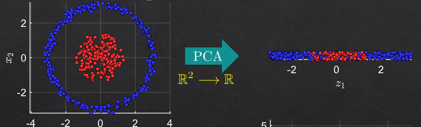
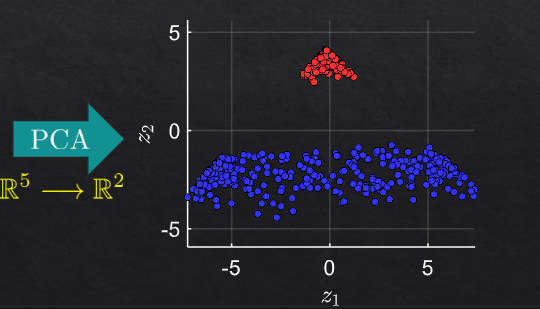
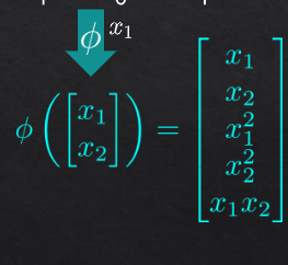
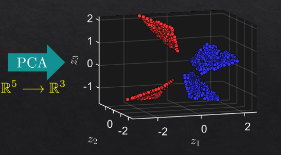
example 1#
for each selected line in the circle:
for transformation to 5 dimensions:
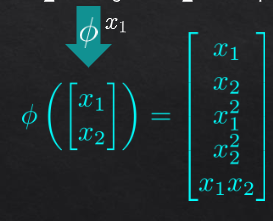
then pca on R5
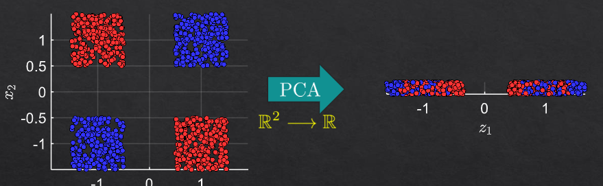
example 2#
Non-Linear PCA and Manifold Learning#
Overview#
Non-Linear PCA (Principal Component Analysis) and Manifold Learning are advanced techniques used in the field of machine learning to reduce the dimensionality of data. While traditional PCA is a linear method, non-linear PCA and manifold learning methods can capture complex, non-linear relationships in the data.
Non-Linear PCA#
Non-Linear PCA extends the concept of traditional PCA to handle non-linear relationships. This is typically done using kernel methods, resulting in Kernel PCA (KPCA).
In Kernel PCA, the data is implicitly mapped to a higher-dimensional feature space using a non-linear mapping. This mapping is done using a kernel function \( k(x, y) \), which computes the dot product in the feature space without explicitly performing the transformation. Common kernel functions include the Gaussian (RBF) kernel and polynomial kernel.
Mathematical Formulation#
Compute the Kernel Matrix: For a given dataset \( X = \{x_1, x_2, \ldots, x_n\} \), compute the kernel matrix \( K \) where \( K_{ij} = k(x_i, x_j) \).
Center the Kernel Matrix: Center \( K \) to have zero mean.
Eigenvalue Decomposition: Perform eigenvalue decomposition on the centered kernel matrix to obtain eigenvalues and eigenvectors.
Projection: Project the original data points onto the principal components in the feature space.
The kernel function \( k(x, y) \) allows the capturing of non-linear relationships in the data.
Manifold Learning#
Manifold learning aims to uncover the low-dimensional structure (manifold) that the high-dimensional data lies on. The key idea is that high-dimensional data often lies on a lower-dimensional manifold embedded in the high-dimensional space.
Popular Manifold Learning Techniques#
t-Distributed Stochastic Neighbor Embedding (t-SNE): Focuses on preserving the local structure of the data by converting pairwise distances into probabilities.
Isomap: Extends MDS (Multidimensional Scaling) to capture non-linear structures by considering geodesic distances (shortest paths on the manifold).
Locally Linear Embedding (LLE): Preserves local neighborhood structures by linearly reconstructing data points from their neighbors.
Mathematical Formulation of Isomap#
Construct the Nearest-Neighbor Graph: Connect each data point to its nearest neighbors based on Euclidean distance.
Compute Geodesic Distances: Use shortest path algorithms (e.g., Dijkstra’s algorithm) to compute the geodesic distances between all pairs of points.
Apply MDS: Apply classical MDS on the geodesic distance matrix to obtain the low-dimensional embedding.
Real-World Examples#
Image Compression: Reducing the dimensionality of high-resolution images to lower dimensions for efficient storage and processing.
Bioinformatics: Analyzing high-dimensional gene expression data to discover underlying biological processes.
Finance: Reducing the complexity of financial data for better visualization and risk management.
Example in Python (Requested)#
Here is a basic example using KernelPCA from the scikit-learn library in Python:
from sklearn.decomposition import KernelPCA
from sklearn.datasets import make_moons
import matplotlib.pyplot as plt

# Generate a toy dataset
X, y = make_moons(n_samples=100, noise=0.1, random_state=42)

# Apply Kernel PCA
kpca = KernelPCA(kernel='rbf', gamma=15)
X_kpca = kpca.fit_transform(X)

# Plot the results
plt.figure(figsize=(8, 6))
plt.scatter(X_kpca[:, 0], X_kpca[:, 1], c=y, cmap='viridis')
plt.title('Kernel PCA with RBF Kernel')
plt.xlabel('Principal Component 1')
plt.ylabel('Principal Component 2')
plt.show()
This example demonstrates how to apply Kernel PCA to a non-linear dataset (make_moons), capturing its intrinsic structure.
In summary, non-linear PCA and manifold learning are powerful tools for dimensionality reduction, especially when dealing with complex, non-linear data. These methods help in uncovering the underlying structure of the data, making it easier to analyze and visualize.