MNIST SVM

Notebook by:

• Royi Avital RoyiAvital@fixelalgorithms.com

Revision History

Version	Date	User	Content / Changes
1.0.000	13/03/2024	Royi Avital	First version

# Import Packages

# General Tools
import numpy as np
import scipy as sp
import pandas as pd

# Machine Learning
from sklearn.datasets import fetch_openml
from sklearn.model_selection import KFold, StratifiedKFold
from sklearn.model_selection import cross_val_predict, train_test_split
from sklearn.svm import LinearSVC, SVC

# Image Processing

# Machine Learning

# Miscellaneous
import math
import os
from platform import python_version
import random
import timeit

# Typing
from typing import Callable, Dict, List, Optional, Set, Tuple, Union

# Visualization
import matplotlib as mpl
import matplotlib.pyplot as plt
import seaborn as sns

# Jupyter
from IPython import get_ipython
from IPython.display import Image
from IPython.display import display
from ipywidgets import Dropdown, FloatSlider, interact, IntSlider, Layout, SelectionSlider
from ipywidgets import interact

Notations

• (?) Question to answer interactively.

• (!) Simple task to add code for the notebook.

• (@) Optional / Extra self practice.

• (#) Note / Useful resource / Food for thought.

Code Notations:

someVar    = 2; #<! Notation for a variable
vVector    = np.random.rand(4) #<! Notation for 1D array
mMatrix    = np.random.rand(4, 3) #<! Notation for 2D array
tTensor    = np.random.rand(4, 3, 2, 3) #<! Notation for nD array (Tensor)
tuTuple    = (1, 2, 3) #<! Notation for a tuple
lList      = [1, 2, 3] #<! Notation for a list
dDict      = {1: 3, 2: 2, 3: 1} #<! Notation for a dictionary
oObj       = MyClass() #<! Notation for an object
dfData     = pd.DataFrame() #<! Notation for a data frame
dsData     = pd.Series() #<! Notation for a series
hObj       = plt.Axes() #<! Notation for an object / handler / function handler

Code Exercise

• Single line fill

vallToFill = ???

• Multi Line to Fill (At least one)

# You need to start writing
????

• Section to Fill

#===========================Fill This===========================#
# 1. Explanation about what to do.
# !! Remarks to follow / take under consideration.
mX = ???

???
#===============================================================#

# Configuration
# %matplotlib inline

seedNum = 512
np.random.seed(seedNum)
random.seed(seedNum)

# Matplotlib default color palette
lMatPltLibclr = ['#1f77b4', '#ff7f0e', '#2ca02c', '#d62728', '#9467bd', '#8c564b', '#e377c2', '#7f7f7f', '#bcbd22', '#17becf']
# sns.set_theme() #>! Apply SeaBorn theme

runInGoogleColab = 'google.colab' in str(get_ipython())

# Constants

FIG_SIZE_DEF    = (8, 8)
ELM_SIZE_DEF    = 50
CLASS_COLOR     = ('b', 'r')
EDGE_COLOR      = 'k'
MARKER_SIZE_DEF = 10
LINE_WIDTH_DEF  = 2

# Courses Packages
import sys
sys.path.append('../')
sys.path.append('../../')
sys.path.append('../../../')
from utils.DataVisualization import PlotConfusionMatrix, PlotLabelsHistogram, PlotMnistImages

# General Auxiliary Functions

Exercise - Cross Validation with the SVM

In this exercise we’ll apply the Cross Validation manually to find the optimal C parameter for the SVM Model.
Instead of using cross_val_predict() we’ll do a manual loop on the folds and average the score.

1. Load the MNIST Data set using fetch_openml().

2. Split the data using Stratified K Fold.

3. For each model (Parameterized by C):

   • Train model on the train sub set.

   • Score model on the test sub set.

4. Plot the score per model.

5. Plot the Confusion Matrix of the best model on the training data.

• (#) Make sure to chose small number of models and folds at the beginning to measure run time and scale accordingly.

• (#) We’ll use LinearSVC class which optimized SVC with kernel linear as it fits for larger data sets.

• (#) You may and should use the functions in the Auxiliary Functions section.

# Parameters

numSamples  = 10_000
numImg = 3

maxItr = 5000 #<! For the LinearSVC model

#===========================Fill This===========================#
# 1. Set the number of folds.
# 1. Set the values of the `C` parameter grid.
numFold = 5
lC = np.linspace(0.001, 1 , 10)
print(lC)
#===============================================================#

# Data Visualization

[0.001 0.112 0.223 0.334 0.445 0.556 0.667 0.778 0.889 1.   ]

Generate / Load Data

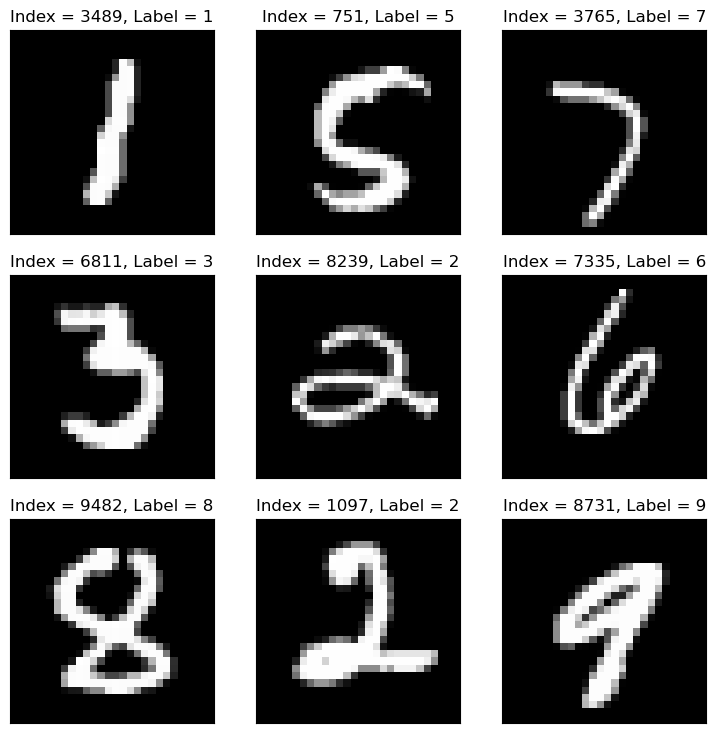
The MNIST database (Modified National Institute of Standards and Technology database) is a large database of handwritten digits.
The MNIST data is a well known data set in Machine Learning, basically it is the Hello World of ML.

The original black and white images from NIST were normalized to fit into a 28x28 pixel bounding box and anti aliased.

• (#) There is an extended version called EMNIST.

# Load Data 

#===========================Fill This===========================#
# 1. Load the MNIST Data using `fetch_openml`.
# !! Use the option `parser = auto`.
mX, vY = fetch_openml('mnist_784', version = 1, return_X_y = True, as_frame = False, parser = 'auto')


vY = vY.astype(np.int_) #<! The labels are strings, convert to integer

#===============================================================#

# The data has many samples, for fast run time we'll sub sample it.

vSampleIdx = np.random.choice(mX.shape[0], numSamples)
mX = mX[vSampleIdx, :]
vY = vY[vSampleIdx]

print(f'The features data shape: {mX.shape}')
print(f'The labels data shape: {vY.shape}')
print(f'The unique values of the labels: {np.unique(vY)}')

The features data shape: (10000, 784)
The labels data shape: (10000,)
The unique values of the labels: [0 1 2 3 4 5 6 7 8 9]

# Pre Process Data
# Scaling the data values.

# The image is in the range {0, 1, ..., 255}.
# We scale it into [0, 1].

#===========================Fill This===========================#
# 1. Scale the features value into the [0, 1] range.
# !! Try implementing it in place.

mX = mX / 255.0

#===============================================================#

Plot Data

# Plot the Data

hF = PlotMnistImages(mX, vY, numImg)

Distribution of Labels

When dealing with classification, it is important to know the balance between the labels within the data set.

# Distribution of Labels

hA = PlotLabelsHistogram(vY)
plt.show()

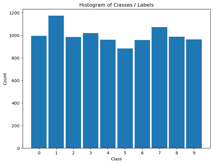
• (?) Looking at the histogram of labels, Is the data balanced?

Cross Validation

The Cross Validation process has 2 main objectives:

1. Estimate the real world performance and its stability.

2. Optimize the model Hyper Parameters.

Cross Validation for Hyper Parameter Optimization

We can also use the Cross Validation approach to search for the best Hype Parameter.
The idea is iterating through the data and measure the score we care about.
The hyper parameter which maximize the score will be used for the production model.

• (?) What kind of a problem is this? Binary Class or Multi Class?

• (?) What kind of strategy will be used? Advise documentation.

• (#) When using LinearSVC:

  • If #Samples > #Features -> Set dual = False.

  • If #Samples < #Features -> Set dual = True (Default).

• (#) If you experience converging issues with LinearSVC use SVC.

print(f"numFold: {numFold}")
print(f"lC: {lC}")

numFold: 5
lC: [0.001 0.112 0.223 0.334 0.445 0.556 0.667 0.778 0.889 1.   ]

# Cross Validation for the C parameter
numC = len(lC)
mACC = np.zeros(shape = (numFold, numC)) #<! Accuracy per Fold and Model

oStrCv = StratifiedKFold(n_splits = numFold, random_state = seedNum, shuffle = True)

for ii, (vTrainIdx, vTestIdx) in enumerate(oStrCv.split(mX, vY)):
    print(f'Working on Fold #{(ii + 1):02d} Out of {numFold} Folds')
    #===========================Fill This===========================#
    # example:
    # numFold = 5 ; len(mX) = 10000 ; len(vY) = 10000
    # 10000 / 5 parts = 2000 each part ;
    # len(vTrainIdx) =    8000  = 4 parts
    # len(vTestIdx) =     2000  = 1 part  

    # Setting the Train / Test split
    mXTrain = mX[vTrainIdx]
    vYTrain = vY[vTrainIdx]
    mXTest  = mX[vTestIdx]
    vYTest  = vY[vTestIdx]
    #===============================================================#
    for jj, C in enumerate(lC):
        print(f'Working on Model #{(jj + 1):02d} Out of {numC} Models with C = {C:0.4f}')
        #===========================Fill This===========================#
        # Set the model, train, score
        # Set `max_iter = maxItr`
        # Set `dual = False`
        
        # oSvmCls     = SVC(C = C, kernel = 'linear')
        oSvmCls     = LinearSVC(C = C, max_iter = maxItr, dual = False)

        oSvmCls     = oSvmCls.fit(mXTrain, vYTrain)
        accScore    = oSvmCls.score(mXTest, vYTest)
        #===============================================================#
        mACC[ii, jj] = accScore

Working on Fold #01 Out of 5 Folds
Working on Model #01 Out of 10 Models with C = 0.0010
Working on Model #02 Out of 10 Models with C = 0.1120
Working on Model #03 Out of 10 Models with C = 0.2230
Working on Model #04 Out of 10 Models with C = 0.3340
Working on Model #05 Out of 10 Models with C = 0.4450
Working on Model #06 Out of 10 Models with C = 0.5560
Working on Model #07 Out of 10 Models with C = 0.6670
Working on Model #08 Out of 10 Models with C = 0.7780
Working on Model #09 Out of 10 Models with C = 0.8890
Working on Model #10 Out of 10 Models with C = 1.0000
Working on Fold #02 Out of 5 Folds
Working on Model #01 Out of 10 Models with C = 0.0010
Working on Model #02 Out of 10 Models with C = 0.1120
Working on Model #03 Out of 10 Models with C = 0.2230
Working on Model #04 Out of 10 Models with C = 0.3340
Working on Model #05 Out of 10 Models with C = 0.4450
Working on Model #06 Out of 10 Models with C = 0.5560
Working on Model #07 Out of 10 Models with C = 0.6670
Working on Model #08 Out of 10 Models with C = 0.7780
Working on Model #09 Out of 10 Models with C = 0.8890
Working on Model #10 Out of 10 Models with C = 1.0000
Working on Fold #03 Out of 5 Folds
Working on Model #01 Out of 10 Models with C = 0.0010
Working on Model #02 Out of 10 Models with C = 0.1120
Working on Model #03 Out of 10 Models with C = 0.2230
Working on Model #04 Out of 10 Models with C = 0.3340
Working on Model #05 Out of 10 Models with C = 0.4450
Working on Model #06 Out of 10 Models with C = 0.5560
Working on Model #07 Out of 10 Models with C = 0.6670
Working on Model #08 Out of 10 Models with C = 0.7780
Working on Model #09 Out of 10 Models with C = 0.8890
Working on Model #10 Out of 10 Models with C = 1.0000
Working on Fold #04 Out of 5 Folds
Working on Model #01 Out of 10 Models with C = 0.0010
Working on Model #02 Out of 10 Models with C = 0.1120
Working on Model #03 Out of 10 Models with C = 0.2230
Working on Model #04 Out of 10 Models with C = 0.3340
Working on Model #05 Out of 10 Models with C = 0.4450
Working on Model #06 Out of 10 Models with C = 0.5560
Working on Model #07 Out of 10 Models with C = 0.6670
Working on Model #08 Out of 10 Models with C = 0.7780
Working on Model #09 Out of 10 Models with C = 0.8890
Working on Model #10 Out of 10 Models with C = 1.0000
Working on Fold #05 Out of 5 Folds
Working on Model #01 Out of 10 Models with C = 0.0010
Working on Model #02 Out of 10 Models with C = 0.1120
Working on Model #03 Out of 10 Models with C = 0.2230
Working on Model #04 Out of 10 Models with C = 0.3340
Working on Model #05 Out of 10 Models with C = 0.4450
Working on Model #06 Out of 10 Models with C = 0.5560
Working on Model #07 Out of 10 Models with C = 0.6670
Working on Model #08 Out of 10 Models with C = 0.7780
Working on Model #09 Out of 10 Models with C = 0.8890
Working on Model #10 Out of 10 Models with C = 1.0000

• (?) How can we accelerate the above calculation?
  Think about dependency between the scores, does it exist?

# Model Score

#===========================Fill This===========================#
# 1. Calculate the score per model (Reduction).
# !! Average over the different folds.

vAvgAcc = np.mean(mACC, axis = 0) #<! Accuracy
print(vAvgAcc)
#===============================================================#

[0.8843 0.8988 0.8956 0.8936 0.8925 0.89   0.8887 0.8879 0.8865 0.8859]

• (?) In the above we used the mean as the reduction operator of many results into one. Can you think on other operators?

• (!) Try using a different reduction method and see results.

# Plot Results

hF, hA = plt.subplots(figsize = FIG_SIZE_DEF)
hA.plot(lC, vAvgAcc)
hA.scatter(lC, vAvgAcc, s = 100)
hA.set_title(f'Accuracy Score as a Function of C - Average of {numFold} Folds')
hA.set_xlabel('C')
hA.set_ylabel('Accuracy')
hA.set_xticks(lC)
hA.grid()

plt.show()

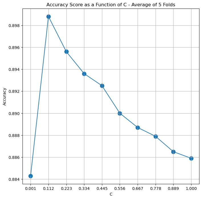
• (?) What range would you choose to do a fine tune over?

Confusion Matrix

The confusion matrix is almost the whole story for classification problems.

Train the model with the best parameter on the whole data and plot the Confusion Matrix.

# Optimal Parameter

#===========================Fill This===========================#
# Extract the optimal C
# Look at `np.argmax()`

optC = lC[np.argmax(vAvgAcc)] #<! Optimal `C` value 
#===============================================================#

print(f'The optimal C value is C = {optC}')

The optimal C value is C = 0.112

# Plot the Confusion Matrix 

#===========================Fill This===========================#
# 1. Build the SVC model with the best parameter.
# 2. Fit & Predict using the model.
# 3. Calculate the accuracy score.
oSvmCls = LinearSVC(C = optC, max_iter = maxItr, dual = False) #<! The model object
oSvmCls = oSvmCls.fit(mX, vY) #<! Fit to data
vYPred = oSvmCls.predict(mX) #<! Predict on the data
dScore = {'Accuracy': np.mean(vYPred == vY)} #<! Dictionary with the `Accuracy` as its key
#===============================================================#

PlotConfusionMatrix(vY, vYPred, dScore = dScore) #<! The accuracy should be >= than above!
plt.show()

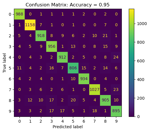
• (?) Is the accuracy above higher or smaller than the one on the cross validation? Why?

• (!) Run the above using SVC() instead of LinearSVC().