Circles Decision Tree Classifier

Circles Decision Tree Classifier#

Notebook by:

Royi Avital RoyiAvital@fixelalgorithms.com

Revision History#

Version	Date	User	Content / Changes
1.0.000	23/03/2024	Royi Avital	First version

# Import Packages

# General Tools
import numpy as np
import scipy as sp
import pandas as pd

# Machine Learning
from sklearn.datasets import make_circles, make_classification
from sklearn.model_selection import train_test_split
from sklearn.tree import DecisionTreeClassifier, plot_tree


# Miscellaneous
import math
import os
from platform import python_version
import random
import timeit

# Typing
from typing import Callable, Dict, List, Optional, Set, Tuple, Union

# Visualization
import matplotlib as mpl
import matplotlib.pyplot as plt
import seaborn as sns

# Jupyter
from IPython import get_ipython
from IPython.display import Image
from IPython.display import display
from ipywidgets import Dropdown, FloatSlider, interact, IntSlider, Layout, SelectionSlider
from ipywidgets import interact

Notations#

(?) Question to answer interactively.
(!) Simple task to add code for the notebook.
(@) Optional / Extra self practice.
(#) Note / Useful resource / Food for thought.

Code Notations:

someVar    = 2; #<! Notation for a variable
vVector    = np.random.rand(4) #<! Notation for 1D array
mMatrix    = np.random.rand(4, 3) #<! Notation for 2D array
tTensor    = np.random.rand(4, 3, 2, 3) #<! Notation for nD array (Tensor)
tuTuple    = (1, 2, 3) #<! Notation for a tuple
lList      = [1, 2, 3] #<! Notation for a list
dDict      = {1: 3, 2: 2, 3: 1} #<! Notation for a dictionary
oObj       = MyClass() #<! Notation for an object
dfData     = pd.DataFrame() #<! Notation for a data frame
dsData     = pd.Series() #<! Notation for a series
hObj       = plt.Axes() #<! Notation for an object / handler / function handler

Code Exercise#

Single line fill

vallToFill = ???

Multi Line to Fill (At least one)

# You need to start writing
????

Section to Fill

#===========================Fill This===========================#
# 1. Explanation about what to do.
# !! Remarks to follow / take under consideration.
mX = ???

???
#===============================================================#

# Configuration
# %matplotlib inline

seedNum = 512
np.random.seed(seedNum)
random.seed(seedNum)

# Matplotlib default color palette
lMatPltLibclr = ['#1f77b4', '#ff7f0e', '#2ca02c', '#d62728', '#9467bd', '#8c564b', '#e377c2', '#7f7f7f', '#bcbd22', '#17becf']
# sns.set_theme() #>! Apply SeaBorn theme

runInGoogleColab = 'google.colab' in str(get_ipython())

# Constants

# Courses Packages
import sys,os
sys.path.append('../')
sys.path.append('../../')
sys.path.append('../../../')
from utils.DataVisualization  import PlotBinaryClassData, PlotDecisionBoundaryClosure

# General Auxiliary Functions

Decision Tree Classifier#

Decision Tree is a graph visualization of a set of decisions.
In the context of Machine Learning the decision are basically limited to a binary decision rule over a single feature.
It means the decision boundary is composed by boxes.

(#) There are extensions to the concept which extends beyond the concept described above.

# Parameters

# Data Generation (1st)
numSamples = 600
noiseLevel = 0.01

# Data Generation (2nd)
numFeatures     = 2 #<! Number of total features
numInformative  = 2 #<! Number of informative features
numRedundant    = 0 #<! Number of redundant features
numRepeated     = 0 #<! Number of repeated features
numClasses      = 2 #<! Number of classes
flipRatio       = 0.05 #<! Number of random swaps

testRatio = 0.25

# Data Visualization
numGridPts = 500

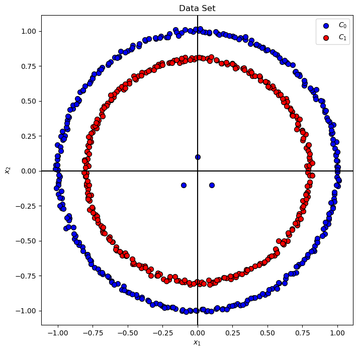
Generate / Load Data#

# Generate Data

mX, vY  = make_circles(n_samples = numSamples, noise = noiseLevel)

mX[0, :] = [0,     0.1]
mX[1, :] = [-0.1, -0.1]
mX[2, :] = [0.1,  -0.1]
vY[:3]   = 0

print(f'The features data shape: {mX.shape}')
print(f'The labels data shape: {vY.shape}')

The features data shape: (600, 2)
The labels data shape: (600,)

Plot Data#

# Plot the Data

# Decision Boundary Plotter
PlotDecisionBoundary = PlotDecisionBoundaryClosure(numGridPts, mX[:, 0].min(), mX[:, 0].max(), mX[:, 1].min(), mX[:, 1].max())

hA = PlotBinaryClassData(mX, vY, axisTitle = 'Data Set')
hA.set_xlabel('${x}_{1}$')
hA.set_ylabel('${x}_{2}$')

plt.show()

../../../_images/c2c98508c489c0bac6db965c49dfdd2d3217462d0d0afdaf8e5ef5b4167898e9.png

Train a Decision Tree Classifier#

Decision trains can easily, with enough degrees of freedom, can easily overfit to data (Represent any data).
Hence tweaking their hyper parameters is crucial.

The decision tree is implemented in the DecisionTreeClassifier class.

(#) The SciKit Learn default for a Decision Tree tend to overfit data.
(#) The max_depth parameter and max_leaf_nodes parameter are usually used exclusively.
(#) We can learn about the data by the orientation of the tree (How balanced it is).
(#) Decision Trees are usually used in the context of ensemble (Random Forests / Boosted Trees).

# Plotting Function

def PlotDecisionTree( splitCriteria, numLeaf, mX: np.ndarray, vY: np.ndarray ):
    
    # Train the classifier
    oTreeCls = DecisionTreeClassifier(criterion = splitCriteria, max_leaf_nodes = numLeaf, random_state = 0)
    oTreeCls = oTreeCls.fit(mX, vY)
    clsScore = oTreeCls.score(mX, vY)
    
    hF, hA = plt.subplots(1, 2, figsize = (16, 8))
    hA = hA.flat
    
    # Decision Boundary
    hA[0] = PlotDecisionBoundary(oTreeCls.predict, hA = hA[0])
    hA[0] = PlotBinaryClassData(mX, vY, hA = hA[0], axisTitle = f'Classifier Decision Boundary, Accuracy = {clsScore:0.2%}')
    hA[0].set_xlabel('${x}_{1}$')
    hA[0].set_ylabel('${x}_{2}$')

    # Plot the Tree
    plot_tree(oTreeCls, filled = True, ax = hA[1], rounded = True)
    hA[1].set_title(f'Max Leaf Nodes = {numLeaf}')

# Plotting Wrapper
hPlotDecisionTree = lambda splitCriteria, numLeaf: PlotDecisionTree(splitCriteria, numLeaf, mX, vY)

# Display the Geometry of the Classifier

splitCriteriaDropdown   = Dropdown(options = ['gini', 'entropy', 'log_loss'], value = 'gini', description = 'Split Criteria')
numLeafSlider           = IntSlider(min = 2, max = 20, step = 1, value = 2, layout = Layout(width = '30%'))
interact(hPlotDecisionTree, splitCriteria = splitCriteriaDropdown, numLeaf = numLeafSlider)

plt.show()

(?) Given K leaves, how many splits are there?

Train & Test Error as a Function of the Degrees of Freedom (DoF) of the Model#

The DoF of the decision tree model is determined by the number of leaves.
In this section we’ll show how the number of leaves effects the performance on the train and test sets.

(?) What kind of behavior of the error of the train set as a function of the number of splits is expected?
(?) What kind of behavior of the error of the test set as a function of the number of splits is expected?

# Generate Data

mXX, vYY = make_classification(n_samples = numSamples, n_features = numFeatures, 
                               n_informative = numInformative, n_redundant = numRedundant, 
                               n_repeated = numRepeated, n_classes = numClasses, flip_y = flipRatio)

print(f'The features data shape: {mXX.shape}')
print(f'The labels data shape: {vYY.shape}')

# Decision Boundary Plotter
PlotDecisionBoundaryXX = PlotDecisionBoundaryClosure(numGridPts, mXX[:, 0].min(), mXX[:, 0].max(), mXX[:, 1].min(), mXX[:, 1].max())

The features data shape: (600, 2)
The labels data shape: (600,)

# Train Test Split

mXTrain, mXTest, vYTrain, vYTest = train_test_split(mXX, vYY, test_size = testRatio, shuffle = True, stratify = vYY)

# Train a Tree

lDecTree  = [DecisionTreeClassifier(max_leaf_nodes = kk, random_state = 0).fit(mXTrain, vYTrain) for kk in range(2, 61)]
vTrainErr = np.array([(1 - oTreeCls.score(mXTrain, vYTrain)) for oTreeCls in lDecTree])
vTestErr  = np.array([(1 - oTreeCls.score(mXTest, vYTest)) for oTreeCls in lDecTree])

# Plotting Function

def PlotDecisionTreeTestTrain( numLeaf, lDecTree, vTrainErr, vTestErr, mXTrain: np.ndarray, vYTrain: np.ndarray, mXTest: np.ndarray, vYTest: np.ndarray ):
    
    numSplits = numLeaf - 1
    
    # The classifier
    oTreeCls = lDecTree[numLeaf - 2]
    
    hF, hA = plt.subplots(1, 3, figsize = (16, 8))
    hA = hA.flat
    
    # Decision Boundary - Train
    hA[0] = PlotDecisionBoundaryXX(oTreeCls.predict, hA = hA[0])
    hA[0] = PlotBinaryClassData(mXTrain, vYTrain, hA = hA[0], axisTitle = f'Train Set, Error Rate = {vTrainErr[numLeaf - 2]:0.2%}')
    hA[0].set_xlabel('${x}_{1}$')
    hA[0].set_ylabel('${x}_{2}$')

    # Decision Boundary - Test
    hA[1] = PlotDecisionBoundaryXX(oTreeCls.predict, hA = hA[1])
    hA[1] = PlotBinaryClassData(mXTest, vYTest, hA = hA[1], axisTitle = f'Test Set, Error Rate = {vTestErr[numLeaf - 2]:0.2%}')
    hA[1].set_xlabel('${x}_{1}$')
    hA[1].set_ylabel('${x}_{2}$')

    # Plot the Error
    yMax = 1.1 * max(vTrainErr.max(), vTestErr.max())
    yMin = 0.9 * min(vTrainErr.min(), vTestErr.min())
    hA[2].plot(range(1, numLeaf), vTrainErr[:numSplits], color = 'm', lw = 2, marker = '.', markersize = 20, label = 'Train Error')
    hA[2].plot(range(1, numLeaf), vTestErr[:numSplits], color = 'k', lw = 2, marker = '.', markersize = 20, label = 'Test Error' )
    hA[2].set_ylim((yMin, yMax))
    hA[2].set_title(f'Max Splits = {numSplits}')
    hA[2].set_xlabel('Number of Leaves')
    hA[2].set_ylabel('Error Rate')
    hA[2].legend()

# Plotting Wrapper
hPlotDecisionTreeTestTrain = lambda numLeaf: PlotDecisionTreeTestTrain(numLeaf, lDecTree, vTrainErr, vTestErr, mXTrain, vYTrain, mXTest, vYTest)

# Display the Geometry of the Classifier

numLeafSlider = IntSlider(min = 2, max = len(lDecTree) + 1, step = 1, value = 2, layout = Layout(width = '30%'))
interact(hPlotDecisionTreeTestTrain, numLeaf = numLeafSlider)

plt.show()

(?) What are the boundaries of the under fit, fit and over fit of the model as a function of the number of splits?