Linear Classifier MOONs

Linear Classifier MOONs#

Notebook by:

Royi Avital RoyiAvital@fixelalgorithms.com

Revision History#

Version	Date	User	Content / Changes
1.0.000	02/03/2024	Royi Avital	First version

# Import Packages

# General Tools
import numpy as np
import scipy as sp
import pandas as pd

# Machine Learning
from sklearn.datasets import make_moons

# Image Processing

# Machine Learning


# Miscellaneous
import os
from platform import python_version
import random
import timeit

# Typing
from typing import Callable, List, Tuple

# Visualization
import matplotlib as mpl
import matplotlib.pyplot as plt
import seaborn as sns
# from bokeh.plotting import figure, show

# Jupyter
from IPython import get_ipython
from IPython.display import Image, display
from ipywidgets import Dropdown, FloatSlider, interact, IntSlider, Layout

Notations#

(?) Question to answer interactively.
(!) Simple task to add code for the notebook.
(@) Optional / Extra self practice.
(#) Note / Useful resource / Food for thought.

Code Notations:

someVar    = 2; #<! Notation for a variable
vVector    = np.random.rand(4) #<! Notation for 1D array
mMatrix    = np.random.rand(4, 3) #<! Notation for 2D array
tTensor    = np.random.rand(4, 3, 2, 3) #<! Notation for nD array (Tensor)
tuTuple    = (1, 2, 3) #<! Notation for a tuple
lList      = [1, 2, 3] #<! Notation for a list
dDict      = {1: 3, 2: 2, 3: 1} #<! Notation for a dictionary
oObj       = MyClass() #<! Notation for an object
dfData     = pd.DataFrame() #<! Notation for a data frame
dsData     = pd.Series() #<! Notation for a series
hObj       = plt.Axes() #<! Notation for an object / handler / function handler

Code Exercise#

Single line fill

vallToFill = ???

Multi Line to Fill (At least one)

# You need to start writing
????

Section to Fill

#===========================Fill This===========================#
# 1. Explanation about what to do.
# !! Remarks to follow / take under consideration.
mX = ???

???
#===============================================================#

# Configuration
# %matplotlib inline

seedNum = 512
np.random.seed(seedNum)
random.seed(seedNum)

# Matplotlib default color palette
lMatPltLibclr = ['#1f77b4', '#ff7f0e', '#2ca02c', '#d62728', '#9467bd', '#8c564b', '#e377c2', '#7f7f7f', '#bcbd22', '#17becf']
# sns.set_theme() #>! Apply SeaBorn theme

runInGoogleColab = 'google.colab' in str(get_ipython())

# Constants

FIG_SIZE_DEF    = (8, 8)
ELM_SIZE_DEF    = 50
CLASS_COLOR     = ('b', 'r')
EDGE_COLOR      = 'k'
MARKER_SIZE_DEF = 10
LINE_WIDTH_DEF  = 2

# Courses Packages
import sys
sys.path.append('../')
sys.path.append('../../')
sys.path.append('../../../')
from utils.DataVisualization import Plot2DLinearClassifier, PlotBinaryClassData

# General Auxiliary Functions

# Parameters

# Data Generation
numSamples = 500
noiseLevel = 0.1

# Data Visualization
numGridPts = 250

Generate / Load Data#

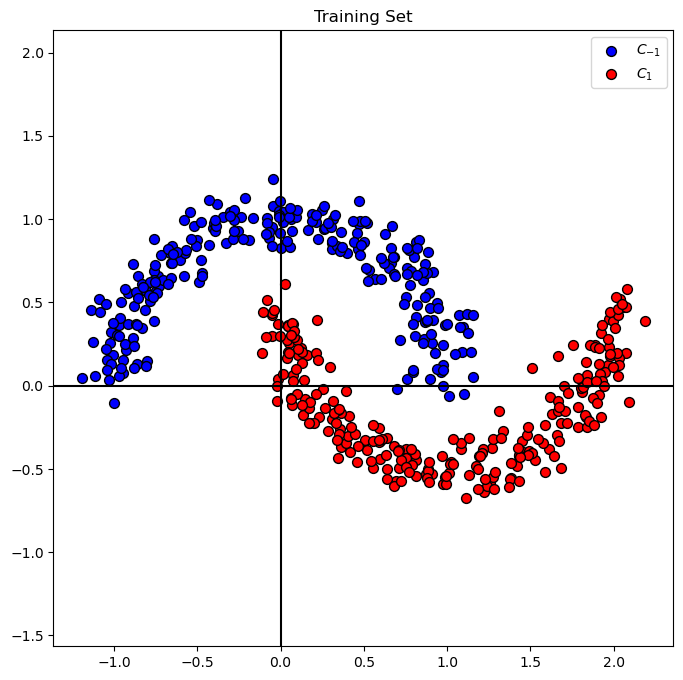
We’ll use the the classic moons data set.
By default it labels the data \({y}_{i} \in \left\{ 0, 1 \right\}\).
We’ll transform it into \({y}_{i} \in \left\{ -1, 1 \right\}\).

# Generate Data 
mX, vY = make_moons(n_samples = numSamples, noise = noiseLevel)

print(f'The features data shape: {mX.shape}')
print(f'The labels data shape: {vY.shape}')

The features data shape: (500, 2)
The labels data shape: (500,)

# The Labels
# The labels of the data
print(f'The unique values of the labels: {np.unique(vY)}')

The unique values of the labels: [0 1]

(?) Do the labels fit the model? What should be done?

# Labels Transformation
# Transforming the Labels into {-1, 1}
vY[vY == 0] = -1

# The Labels
# The updated labels
print(f'The unique values of the labels: {np.unique(vY)}')

The unique values of the labels: [-1  1]

Plot the Data#

# Plot the Data

hA = PlotBinaryClassData(mX, vY, axisTitle = 'Training Set')

../../../../_images/938a10737baeb9a1c939c7da6d45e28644355ee9d15e3c614e47c33c4b53b7ed.png

Linear Classifier Training#

\[ {f}_{\left( \boldsymbol{w} \right)} \left( \boldsymbol{x} \right) = \mathrm{sign} \left( \boldsymbol{w}^{T} \boldsymbol{x} \right) \]

Training Optimization Problem#

In ideal world, we’d like to optimize:

\[ \hat{ \boldsymbol{w} } = \arg \min_{\boldsymbol{w}} {\left\| \operatorname{sign} \left( \boldsymbol{X} \boldsymbol{w} \right) - \boldsymbol{y} \right\|}_{2}^{2} \]

Where

\[\begin{split} \boldsymbol{X} = \begin{bmatrix} -1 & - & x_{1} & -\\ -1 & - & x_{2} & -\\ & \vdots \\ -1 & - & x_{N} & - \end{bmatrix} \in \mathbb{R}^{N \times 3} \end{split}\]

# Stack the constant column into `mX`
mX = np.column_stack((-np.ones(numSamples), mX))
mX

array([[-1.        ,  0.75042724,  0.53523666],
       [-1.        , -0.1674125 ,  1.00862292],
       [-1.        ,  0.22313782,  0.87931898],
       ...,
       [-1.        ,  1.48488659, -0.24967477],
       [-1.        ,  1.59026907, -0.2386105 ],
       [-1.        ,  1.89492566,  0.0257667 ]])

(?) What are the dimensions of mX?

# The updated dimensions
print(f'The features data shape: {mX.shape}')

The features data shape: (500, 3)

Yet, since the \(\operatorname{sign} \left( \cdot \right)\) isn’t smooth nor continuous we need to approximate it.
The classic candidate is the Sigmoid Function (Member of the S Shaped function family):

\[ \sigma \left( x \right) = 2 \frac{ \exp \left( x \right) }{ 1 + \exp \left( x \right) } - 1 = 2 \frac{ 1 }{ 1 + \exp \left( -x \right) } - 1 \]

See scipy.special.expit() for \(\frac{ 1 }{ 1 + \exp \left( -x \right) }\).

(#) In practice such function requires numerical stable implementation. Use professionally made implementations if available.

The Sigmoid Function derivative is given by:

\[ \frac{\mathrm{d} \sigma \left( x \right) }{\mathrm{d} x} = 2 \frac{ \exp \left( x \right)}{\left( 1 + \exp \left( x \right) \right)^{2}} = 2 \left( \frac{ 1 }{ 1 + \exp \left( -x \right) } \right) \left( 1 - \frac{ 1 }{ 1 + \exp \left( -x \right) } \right) \]

(#) For derivation of the last step, see https://math.stackexchange.com/questions/78575.

The Loss Function#

Then, using the Sigmoid approximation the loss function becomes (With mean over all data samples \(N\)):

\[ \hat{ \boldsymbol{w} } = \arg \min_{\boldsymbol{w}} J \left( \boldsymbol{w} \right) = \arg \min_{\boldsymbol{w}} \frac{1}{4 N} {\left\| \sigma \left( \boldsymbol{X} \boldsymbol{w} \right) - \boldsymbol{y} \right\|}_{2}^{2} \]

The gradient becomes:

\[\nabla_{\boldsymbol{w}} J \left( \boldsymbol{w} \right) = \frac{1}{2N} \boldsymbol{X}^{T} \operatorname{Diag} \left( \sigma' \left( \boldsymbol{X} \boldsymbol{w} \right) \right) \left( \sigma \left( \boldsymbol{X} \boldsymbol{w}\right) - \boldsymbol{y} \right) \]

(?) Is the problem convex?
(#) For classification the _Squared \({L}^{2}\) Loss is replaced with Cross Entropy Loss which has better properties in the context of optimization for classification.
(#) For information about the objective function in the context of classification see Stanley Chan - Purdue University - ECE595 / STAT598: Machine Learning I Lecture 14 Logistic Regression.

# Defining the Functions

def SigmoidFun( vX: np.ndarray ):
    
    return (2 * sp.special.expit(vX)) - 1

def GradSigmoidFun(vX: np.ndarray):

    vExpit = sp.special.expit(vX)
    
    return 2 * vExpit * (1 - vExpit)

def LossFun(mX: np.ndarray, vW: np.ndarray, vY: np.ndarray):

    numSamples = mX.shape[0]

    vR = SigmoidFun(mX @ vW) - vY
    
    return np.sum(np.square(vR)) / (4 * numSamples)

def GradLossFun(mX: np.ndarray, vW: np.ndarray, vY: np.ndarray):

    numSamples = mX.shape[0]
    
    return (mX.T * GradSigmoidFun(mX @ vW).T) @ (SigmoidFun(mX @ vW) - vY) / (2 * numSamples)

The Gradient Descent#

\[ \boldsymbol{w}_{k + 1} = \boldsymbol{w}_{k} - \mu \nabla_{\boldsymbol{w}} J \left( \boldsymbol{w}_{k} \right) \]

# Gradient Descent

# Parameters
K   = 1000 #<! Num Steps
µ   = 0.10 #<! Step Size
vW  = np.array([0.0, -1.0, 2.0]) #<! Initial w

mW = np.zeros(shape = (vW.shape[0], K)) #<! Model Parameters (Weights)
vE = np.full(shape = K, fill_value = None) #<! Errors
vL = np.full(shape = K, fill_value = None) #<! Loss

vHatY = np.sign(mX @ vW) #<! Apply the classifier

mW[:, 0]    = vW
vE[0]       = np.mean(vHatY != vY)
vL[0]       = LossFun(mX, vW, vY)

for kk in range(1, K):
    vW -= µ * GradLossFun(mX, vW, vY)
    
    mW[:, kk]   = vW

    vHatY = np.sign(mX @ vW) #<! Apply the classifier
    
    vE[kk]      = np.mean(vHatY != vY) #<! Mean Error
    vL[kk]      = LossFun(mX, vW, vY) #<! Loss Function

# Plotting Function

# Grid of the data support
vV       = np.linspace(-2, 2, numGridPts)
mX1, mX2 = np.meshgrid(vV, vV)

def PlotLinClassTrain(itrIdx, mX, mW, vY, K, µ, vE, vL, mX1, mX2):

    hF, _ = plt.subplots(nrows = 1, ncols = 2, figsize = (12, 6))

    hA1, hA2 = hF.axes[0], hF.axes[1]

    # hA1.cla()
    # hA2.cla()
    
    Plot2DLinearClassifier(mX, vY, mW[:, itrIdx], mX1, mX2, hA1)

    vEE = vE[:itrIdx]
    vLL = vL[:itrIdx]

    hA2.plot(vEE, color = 'k', lw = 2, label = r'$J \left( w \right)$')
    hA2.plot(vLL, color = 'm', lw = 2, label = r'$\tilde{J} \left( w \right)$')
    hA2.set_title('Objective Function')
    hA2.set_xlabel('Iteration Index')
    hA2.set_ylabel('Value')
    hA2.set_xlim((0, K - 1))
    hA2.set_ylim((0, 1))
    hA2.grid()
    hA2.legend()
        
    # hF.canvas.draw()
    plt.show()

# Display the Optimization Path
# hF, hA = plt.subplots(nrows = 1, ncols = 2, figsize = (12, 6))
# hPlotLinClassTrain = lambda itrIdx: PlotLinClassTrain(itrIdx, mX, mW, vY, K, µ, vE, vL, mX1, mX2, hF)
hPlotLinClassTrain = lambda itrIdx: PlotLinClassTrain(itrIdx, mX[:, 1:], mW, vY, K, µ, vE, vL, mX1, mX2)
kSlider = IntSlider(min = 0, max = K - 1, step = 1, value = 0, layout = Layout(width = '30%'))
interact(hPlotLinClassTrain, itrIdx = kSlider)

# plt.show()

<function __main__.<lambda>(itrIdx)>

(!) Optimize the parameters \(K\) and \(\mu\) to achieve accuracy of ~85% with the least steps.