
DBSCAN Demo#
Notebook by:
Royi Avital RoyiAvital@fixelalgorithms.com
Revision History#
Version |
Date |
User |
Content / Changes |
|---|---|---|---|
1.0.000 |
13/04/2024 |
Royi Avital |
First version |
![]()
# Import Packages

# General Tools
import numpy as np
import scipy as sp
import pandas as pd

# Machine Learning
from sklearn.cluster import DBSCAN
from sklearn.datasets import make_moons

# Miscellaneous
import math
import os
from platform import python_version
import random
import timeit

# Typing
from typing import Callable, Dict, List, Optional, Self, Set, Tuple, Union

# Visualization
import matplotlib as mpl
import matplotlib.pyplot as plt
import seaborn as sns

# Jupyter
from IPython import get_ipython
from IPython.display import Image
from IPython.display import display
from ipywidgets import Dropdown, FloatSlider, interact, IntSlider, Layout, SelectionSlider
from ipywidgets import interact
Notations#
(?) Question to answer interactively.
(!) Simple task to add code for the notebook.
(@) Optional / Extra self practice.
(#) Note / Useful resource / Food for thought.
Code Notations:
someVar    = 2; #<! Notation for a variable
vVector    = np.random.rand(4) #<! Notation for 1D array
mMatrix    = np.random.rand(4, 3) #<! Notation for 2D array
tTensor    = np.random.rand(4, 3, 2, 3) #<! Notation for nD array (Tensor)
tuTuple    = (1, 2, 3) #<! Notation for a tuple
lList      = [1, 2, 3] #<! Notation for a list
dDict      = {1: 3, 2: 2, 3: 1} #<! Notation for a dictionary
oObj       = MyClass() #<! Notation for an object
dfData     = pd.DataFrame() #<! Notation for a data frame
dsData     = pd.Series() #<! Notation for a series
hObj       = plt.Axes() #<! Notation for an object / handler / function handler
Code Exercise#
Single line fill
vallToFill = ???
Multi Line to Fill (At least one)
# You need to start writing
????
Section to Fill
#===========================Fill This===========================#
# 1. Explanation about what to do.
# !! Remarks to follow / take under consideration.
mX = ???

???
#===============================================================#
# Configuration
# %matplotlib inline

seedNum = 512
np.random.seed(seedNum)
random.seed(seedNum)

# Matplotlib default color palette
lMatPltLibclr = ['#1f77b4', '#ff7f0e', '#2ca02c', '#d62728', '#9467bd', '#8c564b', '#e377c2', '#7f7f7f', '#bcbd22', '#17becf']
# sns.set_theme() #>! Apply SeaBorn theme

runInGoogleColab = 'google.colab' in str(get_ipython())
# Constants

FIG_SIZE_DEF    = (8, 8)
ELM_SIZE_DEF    = 50
CLASS_COLOR     = ('b', 'r')
EDGE_COLOR      = 'k'
MARKER_SIZE_DEF = 10
LINE_WIDTH_DEF  = 2
# Courses Packages
import sys
sys.path.append('../')
sys.path.append('../../')
sys.path.append('../../../')
from utils.DataVisualization import PlotScatterData
# General Auxiliary Functions

def PlotDBSCAN( mX: np.ndarray, rVal:float, minSamples: int, metricMethod: str, hA: Optional[plt.Axes] = None, figSize: Tuple[int, int] = FIG_SIZE_DEF, markerSize: int = MARKER_SIZE_DEF ) -> plt.Axes:

    if hA is None:
        hF, hA = plt.subplots(figsize = figSize)
    else:
        hF = hA.get_figure()

    vL = DBSCAN(eps = rVal, min_samples = minSamples, metric = metricMethod).fit_predict(mX)
    numClusters = vL.max() + 1

    vIdxC = vL > -1 #<! Clusters
    vIdxN = vL == -1 #<! Noise

    vC = np.unique(vL[vIdxC])
    for ii in range(numClusters):
        vIdx = vL == ii
        hA.scatter(mX[vIdx, 0], mX[vIdx, 1], s = ELM_SIZE_DEF, edgecolor = EDGE_COLOR, label = f'{ii}')

    hA.scatter(mX[vIdxN, 0], mX[vIdxN, 1], s = 2 * ELM_SIZE_DEF, edgecolor = 'r', label = 'Noise')

    # hA.scatter(mX[vIdxC, 0], mX[:, 1], s = ELM_SIZE_DEF, c = vL[vIdxC], edgecolor = EDGE_COLOR)
    # hA.scatter(mX[vIdxN, 0], mX[:, 1], s = ELM_SIZE_DEF, c = vL[vIdxN], edgecolor = EDGE_COLOR)
    # hS = hA.scatter(mX[:, 0], mX[:, 1], s = ELM_SIZE_DEF, c = vL, edgecolor = EDGE_COLOR)
    hA.set_xlabel('${{x}}_{{1}}$')
    hA.set_ylabel('${{x}}_{{2}}$')
    hA.set_title(f'DBSCAN Clustering, Number of Clusters: {numClusters}, Number of Noise Labels: {np.sum(vIdxN)}')
    hA.legend()

    return hA
Clustering by Density#
This notebook demonstrates clustering using the DBSCAN algorithm.
(#) The DBSCAN method approximates the idea of applying the high dimensionality KDE, applying a threshold and finding the connected components.
(#) The DBSCAN method was improved by other methods. Notable mentions: OPTICS Algorithm and HDBSCAN.
The improvements mostly try to better handle varying density among the clusters.
# Parameters

# Data Generation
vNumSamples = [250, 250, 50] #<! Moon 001, Moon 002, Noise

# Model
Generate / Load Data#
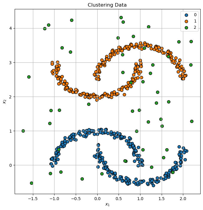
The data is composed on several moon like shaped clusters and noise.
# Generate Data

mX0, _ = make_moons(vNumSamples[0], noise = .05)
mX1, _ = make_moons(vNumSamples[1], noise = .05)
mX1    = mX1 * [1, -1] + [0, 3]
mX2    = np.random.rand(vNumSamples[2], 2) * [4, 5] - [1.75, 2/3]
mX     = np.r_[mX0, mX1, mX2]
vL     = np.repeat(range(len(vNumSamples)), vNumSamples)

print(f'The features data shape: {mX.shape}')
The features data shape: (550, 2)
Plot Data#
# Plot the Data

hF, hA = plt.subplots(figsize = (8, 8))
hA = PlotScatterData(mX, vL, hA = hA)
hA.set_title('Clustering Data');
Cluster Data by DBSCAN#
The DBSCAN method is one of the mor intuitive method (Though tricky to implement efficiently).
It is super powerful and effective, yet requires tweaking of its hyper parameters.
(#) One advantage of the method is the built in support for outliers. Yet, it is not a perfect method (Since noise is not always an outlier!).
(#) As a non parametric method, it doesn’t have built in support for new samples (Out of sample data).
(#) Support for new samples might be done using s supervised model.
(#) It might be tricky with large data sets and high dimensionality.
(#) Implemented in SciKit Learn’s
DBSCANclass.
# Plotting Function Wrapper
hPlotDbscan = lambda rVal, minSamples, metricMethod: PlotDBSCAN(mX, rVal, minSamples, metricMethod, figSize = (7, 7))
# Interactive Visualization

# There are two parameters to the algorithm, `min_samples` and `eps`, which define formally what we mean when we say dense.
# Higher `min_samples` or lower `eps` indicate higher density necessary to form a cluster.

rSlider = FloatSlider(min = 0.05, max = .5, step = 0.05, value = 0.05, layout = Layout(width = '30%'))
zSlider = IntSlider(min = 1, max = 10, step = 1, value = 3, layout = Layout(width = '30%'))
metricMethodDropdown = Dropdown(description = 'Metric Method', options = [('Cityblock', 'cityblock'), ('Cosine', 'cosine'), ('Euclidean', 'euclidean')], value = 'euclidean')
interact(hPlotDbscan, rVal = rSlider, minSamples = zSlider, metricMethod = metricMethodDropdown)

plt.show()