Linear Classifier breast

Notebook by:

• Royi Avital RoyiAvital@fixelalgorithms.com

Revision History

Version	Date	User	Content / Changes
1.0.000	03/03/2024	Royi Avital	First version

# Import Packages

# General Tools
import numpy as np
import scipy as sp
import pandas as pd

# Machine Learning
from sklearn.datasets import load_breast_cancer

# Image Processing

# Machine Learning


# Miscellaneous
import os
from platform import python_version
import random
import timeit

# Typing
from typing import Callable, List, Tuple

# Visualization
import matplotlib as mpl
import matplotlib.pyplot as plt
import seaborn as sns
# from bokeh.plotting import figure, show

# Jupyter
from IPython import get_ipython
from IPython.display import Image, display
from ipywidgets import Dropdown, FloatSlider, interact, IntSlider, Layout

/tmp/ipykernel_1608987/2547312577.py:6: DeprecationWarning: 
Pyarrow will become a required dependency of pandas in the next major release of pandas (pandas 3.0),
(to allow more performant data types, such as the Arrow string type, and better interoperability with other libraries)
but was not found to be installed on your system.
If this would cause problems for you,
please provide us feedback at https://github.com/pandas-dev/pandas/issues/54466
        
  import pandas as pd

Notations

• (?) Question to answer interactively.

• (!) Simple task to add code for the notebook.

• (@) Optional / Extra self practice.

• (#) Note / Useful resource / Food for thought.

Code Notations:

someVar    = 2; #<! Notation for a variable
vVector    = np.random.rand(4) #<! Notation for 1D array
mMatrix    = np.random.rand(4, 3) #<! Notation for 2D array
tTensor    = np.random.rand(4, 3, 2, 3) #<! Notation for nD array (Tensor)
tuTuple    = (1, 2, 3) #<! Notation for a tuple
lList      = [1, 2, 3] #<! Notation for a list
dDict      = {1: 3, 2: 2, 3: 1} #<! Notation for a dictionary
oObj       = MyClass() #<! Notation for an object
dfData     = pd.DataFrame() #<! Notation for a data frame
dsData     = pd.Series() #<! Notation for a series
hObj       = plt.Axes() #<! Notation for an object / handler / function handler

Code Exercise

• Single line fill

vallToFill = ???

• Multi Line to Fill (At least one)

# You need to start writing
????

• Section to Fill

#===========================Fill This===========================#
# 1. Explanation about what to do.
# !! Remarks to follow / take under consideration.
mX = ???

???
#===============================================================#

# Configuration
# %matplotlib inline

seedNum = 512
np.random.seed(seedNum)
random.seed(seedNum)

# Matplotlib default color palette
lMatPltLibclr = ['#1f77b4', '#ff7f0e', '#2ca02c', '#d62728', '#9467bd', '#8c564b', '#e377c2', '#7f7f7f', '#bcbd22', '#17becf']
# sns.set_theme() #>! Apply SeaBorn theme

runInGoogleColab = 'google.colab' in str(get_ipython())

# Constants

FIG_SIZE_DEF    = (8, 8)
ELM_SIZE_DEF    = 50
CLASS_COLOR     = ('b', 'r')
EDGE_COLOR      = 'k'
MARKER_SIZE_DEF = 10
LINE_WIDTH_DEF  = 2

# Courses Packages
import sys
sys.path.append('../../')
from utils.DataVisualization import  Plot2DLinearClassifier, PlotBinaryClassData

# General Auxiliary Functions

# Parameters

# Data Generation


# Data Visualization
numGridPts = 250

Generate / Load Data

We’ll use the Breast Cancer Wisconsin (Diagnostic) Data Set.

• (!) Read about the data and its variables.

# Load / Generate Data 
dData = load_breast_cancer()
mX    = dData.data
vY    = dData.target

print(f'The features data shape: {mX.shape}')
print(f'The labels data shape: {vY.shape}')

The features data shape: (569, 30)
The labels data shape: (569,)

## print some demo data
print(f'First 5 rows of the features data:\n{mX[:5]}')
print(f'First 5 rows of the labels data:\n{vY[:5]}')

First 5 rows of the features data:
[[1.799e+01 1.038e+01 1.228e+02 1.001e+03 1.184e-01 2.776e-01 3.001e-01
  1.471e-01 2.419e-01 7.871e-02 1.095e+00 9.053e-01 8.589e+00 1.534e+02
  6.399e-03 4.904e-02 5.373e-02 1.587e-02 3.003e-02 6.193e-03 2.538e+01
  1.733e+01 1.846e+02 2.019e+03 1.622e-01 6.656e-01 7.119e-01 2.654e-01
  4.601e-01 1.189e-01]
 [2.057e+01 1.777e+01 1.329e+02 1.326e+03 8.474e-02 7.864e-02 8.690e-02
  7.017e-02 1.812e-01 5.667e-02 5.435e-01 7.339e-01 3.398e+00 7.408e+01
  5.225e-03 1.308e-02 1.860e-02 1.340e-02 1.389e-02 3.532e-03 2.499e+01
  2.341e+01 1.588e+02 1.956e+03 1.238e-01 1.866e-01 2.416e-01 1.860e-01
  2.750e-01 8.902e-02]
 [1.969e+01 2.125e+01 1.300e+02 1.203e+03 1.096e-01 1.599e-01 1.974e-01
  1.279e-01 2.069e-01 5.999e-02 7.456e-01 7.869e-01 4.585e+00 9.403e+01
  6.150e-03 4.006e-02 3.832e-02 2.058e-02 2.250e-02 4.571e-03 2.357e+01
  2.553e+01 1.525e+02 1.709e+03 1.444e-01 4.245e-01 4.504e-01 2.430e-01
  3.613e-01 8.758e-02]
 [1.142e+01 2.038e+01 7.758e+01 3.861e+02 1.425e-01 2.839e-01 2.414e-01
  1.052e-01 2.597e-01 9.744e-02 4.956e-01 1.156e+00 3.445e+00 2.723e+01
  9.110e-03 7.458e-02 5.661e-02 1.867e-02 5.963e-02 9.208e-03 1.491e+01
  2.650e+01 9.887e+01 5.677e+02 2.098e-01 8.663e-01 6.869e-01 2.575e-01
  6.638e-01 1.730e-01]
 [2.029e+01 1.434e+01 1.351e+02 1.297e+03 1.003e-01 1.328e-01 1.980e-01
  1.043e-01 1.809e-01 5.883e-02 7.572e-01 7.813e-01 5.438e+00 9.444e+01
  1.149e-02 2.461e-02 5.688e-02 1.885e-02 1.756e-02 5.115e-03 2.254e+01
  1.667e+01 1.522e+02 1.575e+03 1.374e-01 2.050e-01 4.000e-01 1.625e-01
  2.364e-01 7.678e-02]]
First 5 rows of the labels data:
[0 0 0 0 0]

## plot cake graph of vY=0 and vY=1
fig, ax = plt.subplots(1, 1, figsize=FIG_SIZE_DEF)
ax.pie([np.sum(vY == 0), np.sum(vY == 1)], labels=dData.target_names, autopct='%1.1f%%', colors=CLASS_COLOR)
ax.set_title('Proportion of Labels')
plt.show()

## print count of cases
print(f'Number of cases with label 0: {np.sum(vY == 0)}')
print(f'Number of cases with label 1: {np.sum(vY == 1)}')

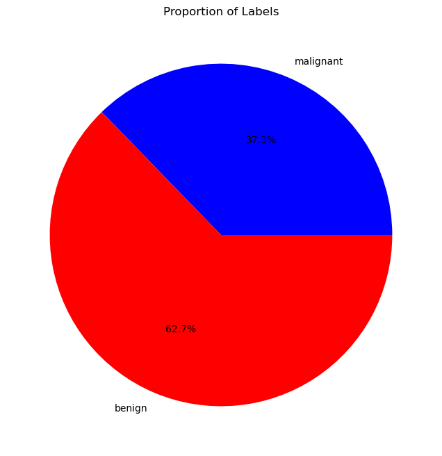
Number of cases with label 0: 212
Number of cases with label 1: 357

# Data Description

print(dData.DESCR)

.. _breast_cancer_dataset:

Breast cancer wisconsin (diagnostic) dataset
--------------------------------------------

**Data Set Characteristics:**

:Number of Instances: 569

:Number of Attributes: 30 numeric, predictive attributes and the class

:Attribute Information:
    - radius (mean of distances from center to points on the perimeter)
    - texture (standard deviation of gray-scale values)
    - perimeter
    - area
    - smoothness (local variation in radius lengths)
    - compactness (perimeter^2 / area - 1.0)
    - concavity (severity of concave portions of the contour)
    - concave points (number of concave portions of the contour)
    - symmetry
    - fractal dimension ("coastline approximation" - 1)

    The mean, standard error, and "worst" or largest (mean of the three
    worst/largest values) of these features were computed for each image,
    resulting in 30 features.  For instance, field 0 is Mean Radius, field
    10 is Radius SE, field 20 is Worst Radius.

    - class:
            - WDBC-Malignant
            - WDBC-Benign

:Summary Statistics:

===================================== ====== ======
                                        Min    Max
===================================== ====== ======
radius (mean):                        6.981  28.11
texture (mean):                       9.71   39.28
perimeter (mean):                     43.79  188.5
area (mean):                          143.5  2501.0
smoothness (mean):                    0.053  0.163
compactness (mean):                   0.019  0.345
concavity (mean):                     0.0    0.427
concave points (mean):                0.0    0.201
symmetry (mean):                      0.106  0.304
fractal dimension (mean):             0.05   0.097
radius (standard error):              0.112  2.873
texture (standard error):             0.36   4.885
perimeter (standard error):           0.757  21.98
area (standard error):                6.802  542.2
smoothness (standard error):          0.002  0.031
compactness (standard error):         0.002  0.135
concavity (standard error):           0.0    0.396
concave points (standard error):      0.0    0.053
symmetry (standard error):            0.008  0.079
fractal dimension (standard error):   0.001  0.03
radius (worst):                       7.93   36.04
texture (worst):                      12.02  49.54
perimeter (worst):                    50.41  251.2
area (worst):                         185.2  4254.0
smoothness (worst):                   0.071  0.223
compactness (worst):                  0.027  1.058
concavity (worst):                    0.0    1.252
concave points (worst):               0.0    0.291
symmetry (worst):                     0.156  0.664
fractal dimension (worst):            0.055  0.208
===================================== ====== ======

:Missing Attribute Values: None

:Class Distribution: 212 - Malignant, 357 - Benign

:Creator:  Dr. William H. Wolberg, W. Nick Street, Olvi L. Mangasarian

:Donor: Nick Street

:Date: November, 1995

This is a copy of UCI ML Breast Cancer Wisconsin (Diagnostic) datasets.
https://goo.gl/U2Uwz2

Features are computed from a digitized image of a fine needle
aspirate (FNA) of a breast mass.  They describe
characteristics of the cell nuclei present in the image.

Separating plane described above was obtained using
Multisurface Method-Tree (MSM-T) [K. P. Bennett, "Decision Tree
Construction Via Linear Programming." Proceedings of the 4th
Midwest Artificial Intelligence and Cognitive Science Society,
pp. 97-101, 1992], a classification method which uses linear
programming to construct a decision tree.  Relevant features
were selected using an exhaustive search in the space of 1-4
features and 1-3 separating planes.

The actual linear program used to obtain the separating plane
in the 3-dimensional space is that described in:
[K. P. Bennett and O. L. Mangasarian: "Robust Linear
Programming Discrimination of Two Linearly Inseparable Sets",
Optimization Methods and Software 1, 1992, 23-34].

This database is also available through the UW CS ftp server:

ftp ftp.cs.wisc.edu
cd math-prog/cpo-dataset/machine-learn/WDBC/

|details-start|
**References**
|details-split|

- W.N. Street, W.H. Wolberg and O.L. Mangasarian. Nuclear feature extraction
  for breast tumor diagnosis. IS&T/SPIE 1993 International Symposium on
  Electronic Imaging: Science and Technology, volume 1905, pages 861-870,
  San Jose, CA, 1993.
- O.L. Mangasarian, W.N. Street and W.H. Wolberg. Breast cancer diagnosis and
  prognosis via linear programming. Operations Research, 43(4), pages 570-577,
  July-August 1995.
- W.H. Wolberg, W.N. Street, and O.L. Mangasarian. Machine learning techniques
  to diagnose breast cancer from fine-needle aspirates. Cancer Letters 77 (1994)
  163-171.

|details-end|

# Features Description

print(dData.feature_names)

['mean radius' 'mean texture' 'mean perimeter' 'mean area'
 'mean smoothness' 'mean compactness' 'mean concavity'
 'mean concave points' 'mean symmetry' 'mean fractal dimension'
 'radius error' 'texture error' 'perimeter error' 'area error'
 'smoothness error' 'compactness error' 'concavity error'
 'concave points error' 'symmetry error' 'fractal dimension error'
 'worst radius' 'worst texture' 'worst perimeter' 'worst area'
 'worst smoothness' 'worst compactness' 'worst concavity'
 'worst concave points' 'worst symmetry' 'worst fractal dimension']

• (#) Fractal Dimension in this context means how curvy and pointy is the perimeter of the object (Digitized image of a fine needle aspirate (FNA) of a breast mass).

# Labels
print(f'The unique values of the labels: {np.unique(vY)}')

The unique values of the labels: [0 1]

# Pre Process Data

# Standardize Data (Features)
# Make each variable: Zero mean, Unit standard deviation / variance
mX = mX - np.mean(mX, axis = 0)
mX = mX / np.std(mX, axis = 0)

# Transforming the Labels into {-1, 1}
vY[vY == 0] = -1

## print 2 line of demo data
print(f'First 2 rows of the features data:\n{mX[:2]}')
print(f'First 2 rows of the labels data:\n{vY[:2]}')

First 2 rows of the features data:
[[ 1.09706398e+00 -2.07333501e+00  1.26993369e+00  9.84374905e-01
   1.56846633e+00  3.28351467e+00  2.65287398e+00  2.53247522e+00
   2.21751501e+00  2.25574689e+00  2.48973393e+00 -5.65265059e-01
   2.83303087e+00  2.48757756e+00 -2.14001647e-01  1.31686157e+00
   7.24026158e-01  6.60819941e-01  1.14875667e+00  9.07083081e-01
   1.88668963e+00 -1.35929347e+00  2.30360062e+00  2.00123749e+00
   1.30768627e+00  2.61666502e+00  2.10952635e+00  2.29607613e+00
   2.75062224e+00  1.93701461e+00]
 [ 1.82982061e+00 -3.53632408e-01  1.68595471e+00  1.90870825e+00
  -8.26962447e-01 -4.87071673e-01 -2.38458552e-02  5.48144156e-01
   1.39236330e-03 -8.68652457e-01  4.99254601e-01 -8.76243603e-01
   2.63326966e-01  7.42401948e-01 -6.05350847e-01 -6.92926270e-01
  -4.40780058e-01  2.60162067e-01 -8.05450380e-01 -9.94437403e-02
   1.80592744e+00 -3.69203222e-01  1.53512599e+00  1.89048899e+00
  -3.75611957e-01 -4.30444219e-01 -1.46748968e-01  1.08708430e+00
  -2.43889668e-01  2.81189987e-01]]
First 2 rows of the labels data:
[-1 -1]

EDA

# combine mx and vy to df
dfData = pd.DataFrame(data = np.c_[mX, vY], columns = np.append(dData.feature_names, 'label'))
sick_data = dfData[dfData['label'] == -1]
healthy_data = dfData[dfData['label'] == 1]

sick_mean = sick_data.mean()
healthy_mean = healthy_data.mean()
## comine the mean of sick and healthy data to new dataframe
dfMean = pd.DataFrame({'sick': sick_mean, 'healthy': healthy_mean})
dfMean

	sick	healthy
mean radius	0.947340	-0.562566
mean texture	0.538776	-0.319945
mean perimeter	0.963700	-0.572281
mean area	0.920031	-0.546349
mean smoothness	0.465295	-0.276309
mean compactness	0.774107	-0.459694
mean concavity	0.903649	-0.536621
mean concave points	1.007793	-0.598465
mean symmetry	0.428880	-0.254685
mean fractal dimension	-0.016659	0.009893
radius error	0.735956	-0.437038
texture error	-0.010775	0.006399
perimeter error	0.721690	-0.428567
area error	0.711432	-0.422475
smoothness error	-0.086965	0.051643
compactness error	0.380218	-0.225788
concavity error	0.329259	-0.195526
concave points error	0.529507	-0.314441
symmetry error	-0.008463	0.005026
fractal dimension error	0.101183	-0.060086
worst radius	1.007585	-0.598342
worst texture	0.592912	-0.352093
worst perimeter	1.015969	-0.603320
worst area	0.952267	-0.565492
worst smoothness	0.546925	-0.324784
worst compactness	0.766924	-0.455428
worst concavity	0.855960	-0.508301
worst concave points	1.029791	-0.611529
worst symmetry	0.540215	-0.320800
worst fractal dimension	0.420281	-0.249579
label	-1.000000	1.000000

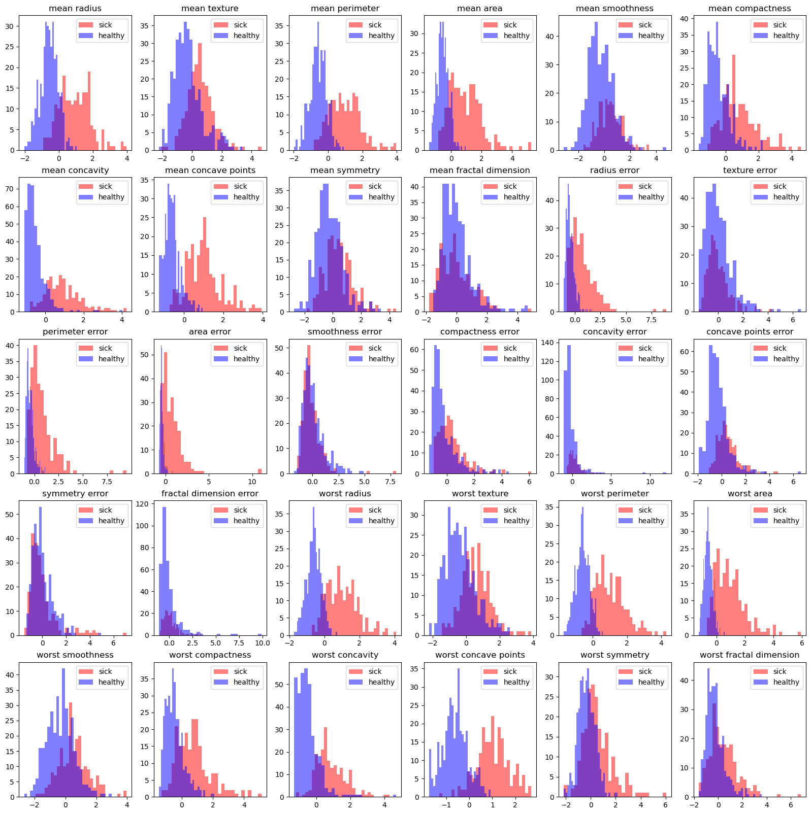
# histogram on every feature
fig, ax = plt.subplots(5, 6, figsize=(20, 20))
for i in range(5):
    for j in range(6):
        ax[i, j].hist(sick_data.iloc[:, i*6+j], bins=30, color='r', alpha=0.5, label='sick')
        ax[i, j].hist(healthy_data.iloc[:, i*6+j], bins=30, color='b', alpha=0.5, label='healthy')
        ax[i, j].set_title(dfData.columns[i*6+j])
        ax[i, j].legend()
plt.show()

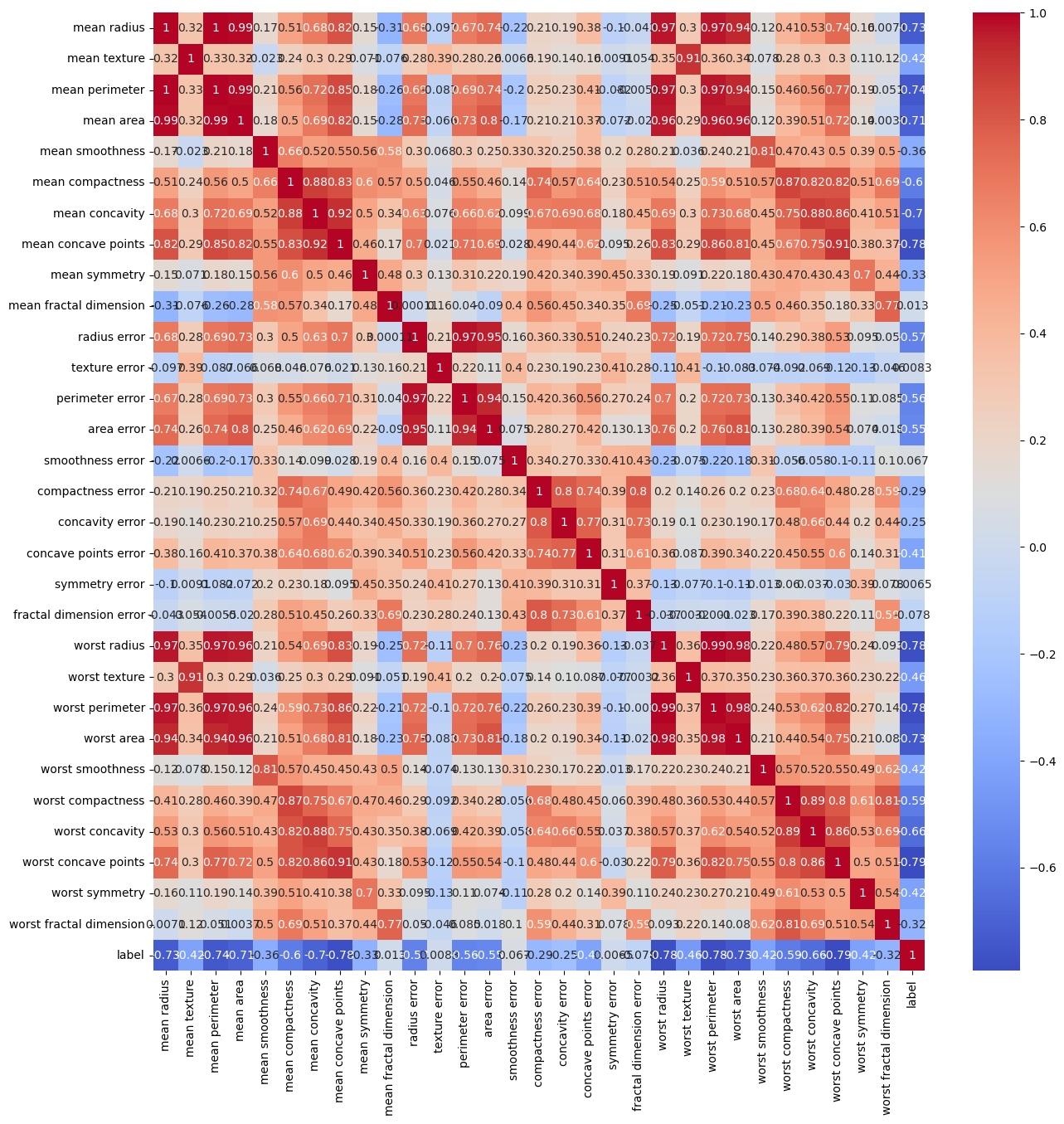
corelation

# heatmap corr with half triangle
fig, ax = plt.subplots(1, 1, figsize=(15, 15))
sns.heatmap(dfData.corr(), annot=True, cmap='coolwarm', ax=ax)
plt.show()

Matrix Form of the Data (Parameterization)

We want to add to the features the constant column:

\[\begin{split} \boldsymbol{X} = \begin{bmatrix} -1 & - & x_{1} & -\\ -1 & - & x_{2} & -\\ & \vdots\\ -1 & - & x_{N} & - \end{bmatrix} \in \mathbb{R}^{N \times 31} \end{split}\]

Tasks:

• (!) Set numSamples to be the number of samples.
  You may find len() / np.shape useful.

• (!) Update mX to the form as above.

Make sure that mX.shape = (569, 31).

#===========================Fill This===========================#
numSamples  = mX.shape[0]
mX          = np.column_stack((-np.ones(numSamples), mX))
#===============================================================#

print(f'numSamples: {numSamples}')
print(f'The features data shape: {mX.shape}') #>! Should be (569, 31)

numSamples: 569
The features data shape: (569, 31)

• (?) Can the data be plotted? Explain.

Calculation Building Blocks

• The Sigmoid Function (Member of the S Shaped function family):

\[ \sigma \left( x \right) = 2 \frac{ \exp \left( x \right) }{ 1 + \exp \left( x \right) } - 1 = 2 \frac{ 1 }{ 1 + \exp \left( -x \right) } - 1 \]

(#) In practice such function requires numerical stable implementation. Use professionally made implementations if available.
(#) See scipy.special.expit() for \(\frac{ 1 }{ 1 + \exp \left( -x \right) }\).

• The gradient of the Sigmoid function:

\[ \frac{\mathrm{d} \sigma \left( x \right) }{\mathrm{d} x} = 2 \frac{ \exp \left( x \right)}{\left( 1 + \exp \left( x \right) \right)^{2}} = 2 \left( \frac{ 1 }{ 1 + \exp \left( -x \right) } \right) \left( 1 - \frac{ 1 }{ 1 + \exp \left( -x \right) } \right) \]

(#) For derivation of the last step, see https://math.stackexchange.com/questions/78575.

• The loss function:

\[ J \left( \boldsymbol{w} \right) = \arg \min_{\boldsymbol{w}} \frac{1}{4 N} {\left\| \sigma \left( \boldsymbol{X} \boldsymbol{w} \right) - \boldsymbol{y} \right\|}_{2}^{2} \]

• The gradient of the loss function:

\[ \nabla_{\boldsymbol{w}} J \left( \boldsymbol{w} \right) = \frac{1}{2N} \boldsymbol{X}^{T} \operatorname{Diag} \left( {\sigma}^{'} \left( \boldsymbol{X} \boldsymbol{w} \right) \right) \left( \sigma \left( \boldsymbol{X} \boldsymbol{w}\right) - \boldsymbol{y} \right) \]

• The accuracy function:

\[ \text{Accuracy} = \frac{1}{N} \sum_{i = 1}^{N} \mathbb{I} \left\{ \hat{y}_{i} = y_{i} \right\}, \; \text{Where} \; \hat{y}_{i} = \operatorname{sign} \left( \boldsymbol{w}^{T} \boldsymbol{x}_{i} \right) \]

• The Gradient Descent step:

\[ \boldsymbol{w}_{k + 1} = \boldsymbol{w}_{k} - \mu \nabla_{\boldsymbol{w}} J \left( \boldsymbol{w}_{k} \right) \]

# Defining the Functions

def SigmoidFun( vX: np.ndarray ) -> np.ndarray:
    
    return (2 * sp.special.expit(vX)) - 1

def GradSigmoidFun(vX: np.ndarray) -> np.ndarray:

    vExpit = sp.special.expit(vX)
    
    return 2 * vExpit * (1 - vExpit)

def LossFun(mX: np.ndarray, vW: np.ndarray, vY: np.ndarray):

    numSamples = mX.shape[0]

    vR = SigmoidFun(mX @ vW) - vY
    
    return np.sum(np.square(vR)) / (4 * numSamples)

def GradLossFun(mX: np.ndarray, vW: np.ndarray, vY: np.ndarray) -> np.ndarray:

    numSamples = mX.shape[0]
    
    return (mX.T * GradSigmoidFun(mX @ vW).T) @ (SigmoidFun(mX @ vW) - vY) / (2 * numSamples)

def CalcAccuracy(mX: np.ndarray, vW: np.ndarray, vY: np.ndarray):
    
    vHatY = np.sign(mX @ vW)
    
    return np.mean(vHatY == vY)

Training the Model (Linear Classifier for Binary Classification)

In this section we’ll implement the training phase using Gradient Descent.

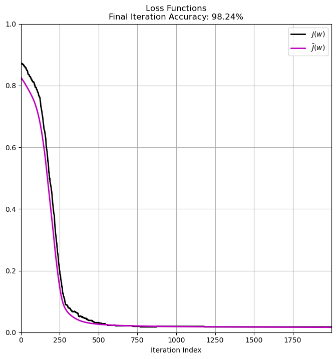
Remark: You should get ~98%.

• (#) Pay attention to the function CalcAccuracy(). You may use it.

# Parameters

#===========================Fill This===========================#
K   = 2000 #<! Num Steps
µ   = 0.1 #<! Step Size
vW  = np.random.rand(31)
print(f'Initial weights: {vW}')
 #<! Initial w
#===============================================================#

mW = np.zeros(shape = (vW.shape[0], K)) #<! Model Parameters (Weights)
vE = np.full(shape = K, fill_value = None) #<! Errors
vL = np.full(shape = K, fill_value = None) #<! Loss

mW[:, 0]    = vW
vE[0]       = 1 - CalcAccuracy(mX, vW, vY)
vL[0]       = LossFun(mX, vW, vY)

#===========================Fill This===========================#
for kk in range(1, K):
    vW -= µ * GradLossFun(mX,vW,vY)   #<! Update the weights

    mW[:, kk] = vW
    
    vE[kk] = 1 - CalcAccuracy(mX, vW, vY) #<! Calculate the mean error
    vL[kk] = LossFun(mX, vW, vY) #<! Calculate the loss
#===============================================================#
    
print(f'Final weights: {vW}')

Initial weights: [0.10729586 0.21193693 0.38785171 0.3651425  0.0847786  0.32761275
 0.46994676 0.55937557 0.26139615 0.78219619 0.61786047 0.9017219
 0.80345349 0.02748905 0.67072269 0.44188427 0.96106932 0.33655362
 0.98704907 0.42054738 0.11551123 0.11973692 0.54273345 0.89399355
 0.62676463 0.30810329 0.76770288 0.58571476 0.49516682 0.53606378
 0.73954955]
Final weights: [-0.55225193 -0.62583161 -0.68353507 -0.48754118 -0.77797179 -0.2619799
 -0.14713312 -0.59526531 -0.88866094 -0.04635121  0.56947724 -0.29342642
  0.29577631 -1.02297835 -0.30874225 -0.07971019  0.6639906  -0.19054818
  0.20944012  0.13290115  0.0185641  -0.99846948 -0.86781874 -0.19301151
 -0.45887152 -0.79122481  0.00341105 -0.5787303  -0.72154294 -0.63409807
  0.09299431]

# Plot the Results

accFinal = CalcAccuracy(mX, vW, vY)

hF, hA = plt.subplots(figsize = FIG_SIZE_DEF)

hA.plot(vE, color = 'k', lw = 2, label = r'$J \left( w \right)$')
hA.plot(vL, color = 'm', lw = 2, label = r'$\tilde{J} \left( w \right)$')
hA.set_title(f'Loss Functions\nFinal Iteration Accuracy: {CalcAccuracy(mX, vW, vY):0.2%}')
hA.set_xlabel('Iteration Index')
hA.set_xlim((0, K - 1))
hA.set_ylim((0, 1))
hA.grid()
hA.legend()
    
plt.show()

for feature in dData.feature_names:
    print(f'{feature} : {vW[dData.feature_names.tolist().index(feature)]}')

mean radius : -0.5522519280612184
mean texture : -0.6258316138842764
mean perimeter : -0.683535065976039
mean area : -0.4875411750013253
mean smoothness : -0.7779717860179926
mean compactness : -0.26197989966146823
mean concavity : -0.14713312309050885
mean concave points : -0.5952653131697615
mean symmetry : -0.8886609449473933
mean fractal dimension : -0.046351209801405426
radius error : 0.5694772434857023
texture error : -0.2934264190691419
perimeter error : 0.2957763108282323
area error : -1.0229783494443443
smoothness error : -0.3087422516592806
compactness error : -0.07971018599884573
concavity error : 0.6639906017559701
concave points error : -0.19054818287282924
symmetry error : 0.20944012391051722
fractal dimension error : 0.132901152234875
worst radius : 0.018564095750620957
worst texture : -0.9984694834556983
worst perimeter : -0.8678187429253742
worst area : -0.19301151234270797
worst smoothness : -0.4588715178248742
worst compactness : -0.7912248088189952
worst concavity : 0.0034110548110386787
worst concave points : -0.5787303037264143
worst symmetry : -0.7215429426871859
worst fractal dimension : -0.6340980726428457

Validate the Gradient Calculation

In order to verify the gradient calculation one may compare it to a numeric approximation of the gradient.
Usually this is done using the classic Finite Difference Method.
Yet this method requires setting the step size parameter (The h parameters in Wikipedia). Its optimal value depends on \(x\) and the function itself.

Yet there is a nice trick called Complex Step Differentiation which goes like:

\[ \frac{\mathrm{d} f \left( x \right) }{\mathrm{d} x} \approxeq \frac{1}{\varepsilon} \Im \left[ f \left( x + i \varepsilon \right) \right] \]

This approximation is less sensitive to the choice of the step size \(\varepsilon\).

• (#) The tricky part of this method is the complex extension of the functions.
  for instance, instead of np.sum(np.abs(vX)) use np.sum(np.sqrt(vX ** 2)).

• (#) Usually setting ε = 1e-8 will do the work.

---

see the complex trick on 01_mathIntro/matCalc/numericAlternative/0007NumericDiff.ipynb

---

# Numerical Calculation of the Gradient by the Complex Step Trick

def CalcFunGrad( hF, vX, ε = 1e-8 ):

    numElements = vX.shape[0]
    
    vY = hF(vX)
    vG = np.zeros(numElements) #<! Gradient
    vP = np.zeros(numElements) #<! Perturbation
    vZ = np.array(vX, dtype = complex)

    for ii in range(numElements):
        vP[ii]  = ε
        vZ.imag = vP
        vG[ii]  = np.imag(hF(vZ)) / ε
        vP[ii]  = 0
    
    return vG

# Updating Functions to Support Complex Input

def SigFunComplex( vX: np.ndarray ) -> np.ndarray:

    return 1 / (1 + np.exp(-vX))


def SigmoidFunComplex( vX: np.ndarray ) -> np.ndarray:
    
    return (2 * SigFunComplex(vX)) - 1


def LossFunComplex(mX: np.ndarray, vW: np.ndarray, vY: np.ndarray):

    numSamples = mX.shape[0]

    vR = SigmoidFunComplex(mX @ vW) - vY
    
    return np.sum(np.square(vR)) / (4 * numSamples)

# Calculating the Gradient Numerically

ε = 1e-8
 
hL = lambda vW: LossFunComplex(mX, vW, vY)

vW = np.random.rand(mX.shape[1])
vG = CalcFunGrad(hL, vW, ε) #<! Numerical gradient

# Verifying the complex variation of the loss function matches the reference 

maxError = np.max(np.abs(LossFunComplex(mX, vW, vY) - LossFun(mX, vW, vY)))
print(f'The maximum absolute deviation of the complex variation: {maxError}')

The maximum absolute deviation of the complex variation: 0.0

# Verifying the analytic gradient vs. the complex step differentiation

maxError = np.max(np.abs(GradLossFun(mX, vW, vY) - vG))
print(f'The maximum absolute deviation of the numerical gradient: {maxError}') #<! We expect it to be less than 1e-8 for Float64

The maximum absolute deviation of the numerical gradient: 1.734723475976807e-17