Random Forests

Random Forests#

Notebook by:

Royi Avital RoyiAvital@fixelalgorithms.com

Revision History#

Version	Date	User	Content / Changes
1.0.000	08/04/2024	Royi Avital	First version

# Import Packages

# General Tools
import numpy as np
import scipy as sp
import pandas as pd

# Machine Learning
from sklearn.datasets import fetch_openml
from sklearn.ensemble import RandomForestClassifier
from sklearn.inspection import permutation_importance
from sklearn.model_selection import train_test_split

# Miscellaneous
import math
import os
from platform import python_version
import random
import timeit

# Typing
from typing import Callable, Dict, List, Optional, Self, Set, Tuple, Union

# Visualization
import matplotlib as mpl
import matplotlib.pyplot as plt
import seaborn as sns

# Jupyter
from IPython import get_ipython
from IPython.display import Image
from IPython.display import display
from ipywidgets import Dropdown, FloatSlider, interact, IntSlider, Layout, SelectionSlider
from ipywidgets import interact

Notations#

(?) Question to answer interactively.
(!) Simple task to add code for the notebook.
(@) Optional / Extra self practice.
(#) Note / Useful resource / Food for thought.

Code Notations:

someVar    = 2; #<! Notation for a variable
vVector    = np.random.rand(4) #<! Notation for 1D array
mMatrix    = np.random.rand(4, 3) #<! Notation for 2D array
tTensor    = np.random.rand(4, 3, 2, 3) #<! Notation for nD array (Tensor)
tuTuple    = (1, 2, 3) #<! Notation for a tuple
lList      = [1, 2, 3] #<! Notation for a list
dDict      = {1: 3, 2: 2, 3: 1} #<! Notation for a dictionary
oObj       = MyClass() #<! Notation for an object
dfData     = pd.DataFrame() #<! Notation for a data frame
dsData     = pd.Series() #<! Notation for a series
hObj       = plt.Axes() #<! Notation for an object / handler / function handler

Code Exercise#

Single line fill

vallToFill = ???

Multi Line to Fill (At least one)

# You need to start writing
????

Section to Fill

#===========================Fill This===========================#
# 1. Explanation about what to do.
# !! Remarks to follow / take under consideration.
mX = ???

???
#===============================================================#

# Configuration
# %matplotlib inline

seedNum = 512
np.random.seed(seedNum)
random.seed(seedNum)

# Matplotlib default color palette
lMatPltLibclr = ['#1f77b4', '#ff7f0e', '#2ca02c', '#d62728', '#9467bd', '#8c564b', '#e377c2', '#7f7f7f', '#bcbd22', '#17becf']
# sns.set_theme() #>! Apply SeaBorn theme

runInGoogleColab = 'google.colab' in str(get_ipython())

# Constants

FIG_SIZE_DEF    = (8, 8)
ELM_SIZE_DEF    = 50
CLASS_COLOR     = ('b', 'r')
EDGE_COLOR      = 'k'
MARKER_SIZE_DEF = 10
LINE_WIDTH_DEF  = 2

# Courses Packages

# General Auxiliary Functions

Random Forests Classification#

In this note book we’ll use the Random Forests based classifier in the task of estimating whether a passenger on the Titanic will or will not survive.
We’ll focus on basic pre processing of the data and analyzing the importance of features using the classifier.

(#) This is a very popular data set for classification. You may have a look for notebooks on the need with a deeper analysis of the data set itself.

# Parameters

# Data
trainRatio = 0.75

# Model
numEst = 150
spliCrit = 'gini'
maxLeafNodes = 20
outBagScore = True

# Feature Permutation
numRepeats = 50

Generate / Load Data#

# Load Data

dfX, dsY = fetch_openml('titanic', version = 1, return_X_y = True, as_frame = True, parser = 'auto')

print(f'The features data shape: {dfX.shape}')
print(f'The labels data shape: {dsY.shape}')

The features data shape: (1309, 13)
The labels data shape: (1309,)

Plot Data#

# Plot the Data

# The Data Frame of Features
dfX.head(10)

	pclass	name	sex	age	sibsp	parch	ticket	fare	cabin	embarked	boat	body	home.dest
0	1	Allen, Miss. Elisabeth Walton	female	29.0000	0	0	24160	211.3375	B5	S	2	NaN	St Louis, MO
1	1	Allison, Master. Hudson Trevor	male	0.9167	1	2	113781	151.5500	C22 C26	S	11	NaN	Montreal, PQ / Chesterville, ON
2	1	Allison, Miss. Helen Loraine	female	2.0000	1	2	113781	151.5500	C22 C26	S	NaN	NaN	Montreal, PQ / Chesterville, ON
3	1	Allison, Mr. Hudson Joshua Creighton	male	30.0000	1	2	113781	151.5500	C22 C26	S	NaN	135.0	Montreal, PQ / Chesterville, ON
4	1	Allison, Mrs. Hudson J C (Bessie Waldo Daniels)	female	25.0000	1	2	113781	151.5500	C22 C26	S	NaN	NaN	Montreal, PQ / Chesterville, ON
5	1	Anderson, Mr. Harry	male	48.0000	0	0	19952	26.5500	E12	S	3	NaN	New York, NY
6	1	Andrews, Miss. Kornelia Theodosia	female	63.0000	1	0	13502	77.9583	D7	S	10	NaN	Hudson, NY
7	1	Andrews, Mr. Thomas Jr	male	39.0000	0	0	112050	0.0000	A36	S	NaN	NaN	Belfast, NI
8	1	Appleton, Mrs. Edward Dale (Charlotte Lamson)	female	53.0000	2	0	11769	51.4792	C101	S	D	NaN	Bayside, Queens, NY
9	1	Artagaveytia, Mr. Ramon	male	71.0000	0	0	PC 17609	49.5042	NaN	C	NaN	22.0	Montevideo, Uruguay

(?) What kind of a feature is name? Should it be used?
(?) What kind of a feature is ticket? Should it be used?

Pre Processing and EDA#

# Dropping Features
# Dropping the `name` and `ticket` features (Avoid 1:1 identification)

dfX = dfX.drop(columns = ['name', 'ticket'])

(#) Pay attention that we dropped the features, but a deeper analysis could extract information from them (Type of ticket, families, etc…).

# The Features Data Frame
dfX.head(10)

	pclass	sex	age	sibsp	parch	fare	cabin	embarked	boat	body	home.dest
0	1	female	29.0000	0	0	211.3375	B5	S	2	NaN	St Louis, MO
1	1	male	0.9167	1	2	151.5500	C22 C26	S	11	NaN	Montreal, PQ / Chesterville, ON
2	1	female	2.0000	1	2	151.5500	C22 C26	S	NaN	NaN	Montreal, PQ / Chesterville, ON
3	1	male	30.0000	1	2	151.5500	C22 C26	S	NaN	135.0	Montreal, PQ / Chesterville, ON
4	1	female	25.0000	1	2	151.5500	C22 C26	S	NaN	NaN	Montreal, PQ / Chesterville, ON
5	1	male	48.0000	0	0	26.5500	E12	S	3	NaN	New York, NY
6	1	female	63.0000	1	0	77.9583	D7	S	10	NaN	Hudson, NY
7	1	male	39.0000	0	0	0.0000	A36	S	NaN	NaN	Belfast, NI
8	1	female	53.0000	2	0	51.4792	C101	S	D	NaN	Bayside, Queens, NY
9	1	male	71.0000	0	0	49.5042	NaN	C	NaN	22.0	Montevideo, Uruguay

# The Labels Data Series
dsY.head(10)

  1
  1
  0
  0
  0
  1
  1
  0
  1
  0
Name: survived, dtype: category
Categories (2, object): ['0', '1']

# Merging Data
dfData = pd.concat([dfX, dsY], axis = 1)

# Data Frame Info
dfData.info()

<class 'pandas.core.frame.DataFrame'>
RangeIndex: 1309 entries, 0 to 1308
Data columns (total 12 columns):
 #   Column     Non-Null Count  Dtype   
---  ------     --------------  -----   
 0   pclass     1309 non-null   int64   
 1   sex        1309 non-null   category
 2   age        1046 non-null   float64 
 3   sibsp      1309 non-null   int64   
 4   parch      1309 non-null   int64   
 5   fare       1308 non-null   float64 
 6   cabin      295 non-null    object  
 7   embarked   1307 non-null   category
 8   boat       486 non-null    object  
 9   body       121 non-null    float64 
 10  home.dest  745 non-null    object  
 11  survived   1309 non-null   category
dtypes: category(3), float64(3), int64(3), object(3)
memory usage: 96.4+ KB

# Missing / Invalid Values
# Null / NA / NaN Matrix

#===========================Fill This===========================#
# 1. Calculate the logical map of invalid values using the method `isna()`.
mInvData = dfData.isna() #<! The logical matrix of invalid values
#===============================================================#

hF, hA = plt.subplots(figsize = FIG_SIZE_DEF)
sns.heatmap(data = mInvData, square = False, ax = hA)
hA.set_title('Invalid Data Map')

plt.show()

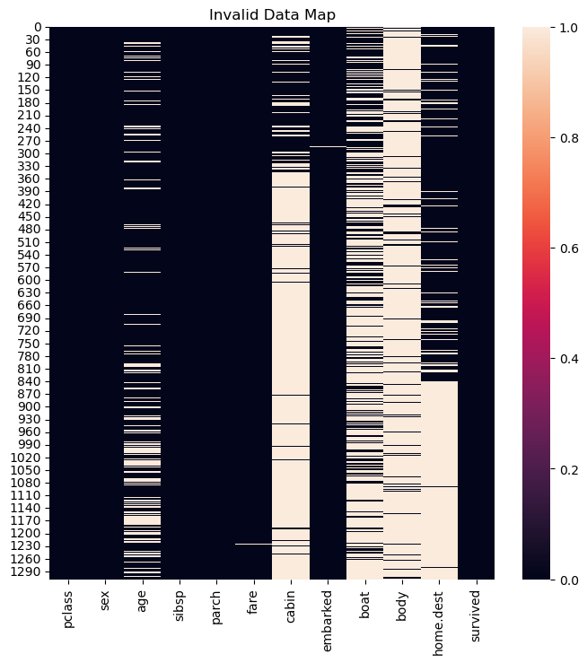
../../../../_images/caab5f7cd5583b7b3d91e190cd2e97bf8a188ee36fecb3f4081772683770a071.png

Since the features cabin, boat, body and home.dest have mostly non valid values the will be dropped as well.

(#) Some implementation of Ensemble Trees can handle missing values. They might benefit in such case asl well.

# Features Filtering
# Removing Features with Invalid Values.

dfData = dfData.drop(columns = ['cabin', 'boat', 'body', 'home.dest'])

# Data Visualization
# Basic EDA on the Data

numCol = dfData.shape[1]
lCols  = dfData.columns
numAx  = int(np.ceil(np.sqrt(numCol)))

# hIsCatLikData = lambda dsX: (pd.api.types.is_categorical_dtype(dsX) or pd.api.types.is_bool_dtype(dsX) or pd.api.types.is_object_dtype(dsX) or pd.api.types.is_integer_dtype(dsX)) #<! Deprecated
hIsCatLikData = lambda dsX: (isinstance(dsX.dtype, pd.CategoricalDtype) or pd.api.types.is_bool_dtype(dsX) or pd.api.types.is_object_dtype(dsX) or pd.api.types.is_integer_dtype(dsX))

hF, hAs = plt.subplots(nrows = numAx, ncols = numAx, figsize = (16, 12))
hAs = hAs.flat

for ii in range(numCol):
    colName = dfData.columns[ii]
    if hIsCatLikData(dfData[colName]):
        sns.histplot(data = dfData, x = colName, hue = 'survived', stat = 'count', discrete = True, common_norm = True, multiple = 'dodge', ax = hAs[ii])
    else:
        sns.kdeplot(data = dfData, x = colName, hue = 'survived', fill = True, common_norm = True, ax = hAs[ii])

plt.show()

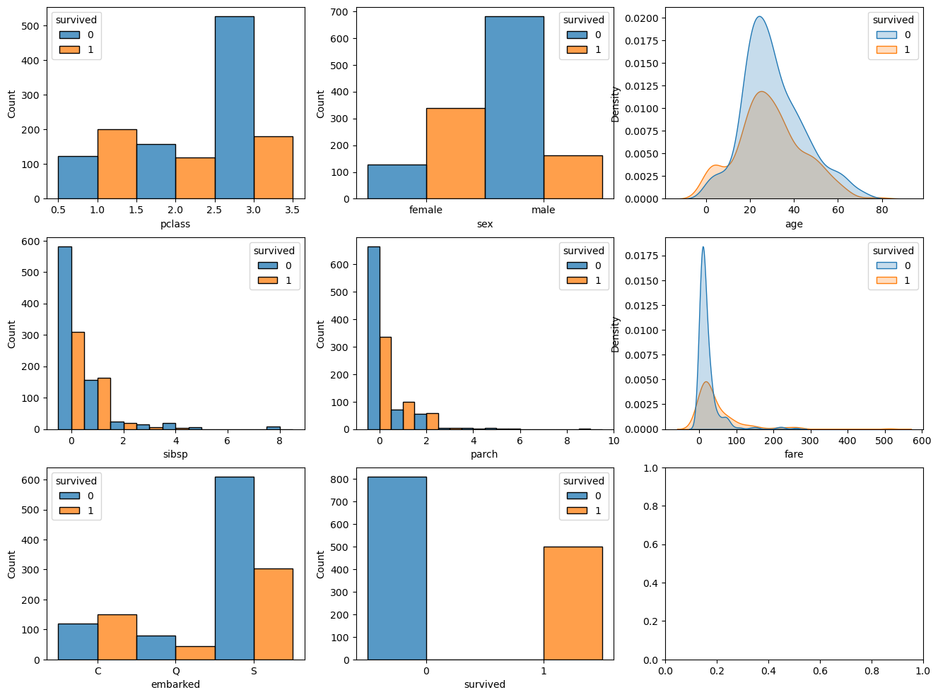
../../../../_images/fbdf0e45388a792ba0bfa9f510f8730a7cbdbd6fd9a5fb7e264f5130d38d8584.png

(?) Have a look on the features and try to estimate their importance for the estimation.

Filling Missing Data#

For the rest of the missing values we’ll use a simple method of interpolation:

Categorical Data: Using the mode value.
Numeric Data: Using the median / mean.

(#) We could employ much more delicate and sophisticated data.
For instance, use the mean value of the same pclass. Namely profiling the data by other features to interpolate the missing feature.
(#) Data imputing can be done by using a model as well: Regression for continuous data, Classification for categorical data.
(#) The relevant classed in SciKti Learn: SimpleImputer, IterativeImputer, KNNImputer.

# Missing Value by Dictionary
dNaNs = {'embarked': dfData['embarked'].mode()[0], 'age': dfData['age'].median(), 'fare': dfData['fare'].median()}

dfData = dfData.fillna(value = dNaNs, inplace = False) #<! We can use the `inplace` for efficiency

(#) The above is equivalent of using SimpleImputer.

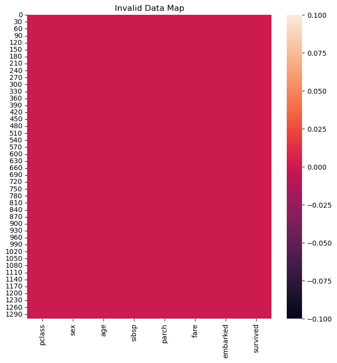
# Null / NA / NaN Matrix

mInvData = dfData.isna() #<! The logical matrix of invalid values

hF, hA = plt.subplots(figsize = FIG_SIZE_DEF)
sns.heatmap(data = mInvData, square = False, ax = hA)
hA.set_title('Invalid Data Map')

plt.show()

../../../../_images/e3a70a8cf1a2e8342057f3acc3f1bf067fe19472748f053d6c1b5d03e163a6c4.png

Conversion of Categorical Data#

In this notebook we’ll use the RandomForestClassifier implementation of Random Forests.
At the moment, it doesn’t support Categorical Data, hence we’ll use Dummy Variables (One Hot Encoding).

(#) Pay attention that one hot encoding is an inferior approach to having a real support for categorical data.
(#) For 2 values categorical data (Binary feature) there is no need fo any special support.
(#) Currently, the implementation of DecisionTreeClassifier doesn’t support categorical values which are not ordinal (As it treats them as numeric). Hence we must use OneHotEncoder.
See status at scikit-learn/scikit-learn#12866.
(#) The One Hot Encoding is not perfect. See Are Categorical Variables Getting Lost in Your Random Forests (Also Notebook - Are Categorical Variables Getting Lost in Your Random Forests).

# Features Encoding
# 1. The feature 'embarked' -> One Hot Encoding.
# 1. The feature 'sex' -> Mapping (Female -> 0, Male -> 1).
dfData = pd.get_dummies(dfData, columns = ['embarked'], drop_first = False)
dfData['sex'] = dfData['sex'].map({'female': 0, 'male': 1})

# Convert Data Type
dfData = dfData.astype(dtype = {'pclass': np.uint8, 'sex': np.uint8, 'sibsp': np.uint8, 'parch': np.uint8, 'survived': np.uint8})

dfData.info()

<class 'pandas.core.frame.DataFrame'>
RangeIndex: 1309 entries, 0 to 1308
Data columns (total 10 columns):
 #   Column      Non-Null Count  Dtype  
---  ------      --------------  -----  
 0   pclass      1309 non-null   uint8  
 1   sex         1309 non-null   uint8  
 2   age         1309 non-null   float64
 3   sibsp       1309 non-null   uint8  
 4   parch       1309 non-null   uint8  
 5   fare        1309 non-null   float64
 6   survived    1309 non-null   uint8  
 7   embarked_C  1309 non-null   bool   
 8   embarked_Q  1309 non-null   bool   
 9   embarked_S  1309 non-null   bool   
dtypes: bool(3), float64(2), uint8(5)
memory usage: 30.8 KB

Train the Random Forests Model#

The random forests models basically creates weak classifiers by limiting their access to the data and features.
This basically also limits their correlation which means we can use their mean in order to reduce the variance of the estimation.

Split Train & Test#

# Split to Features and Labels

dfX = dfData.drop(columns = ['survived'])
dsY = dfData['survived']

print(f'The features data shape: {dfX.shape}')
print(f'The labels data shape: {dsY.shape}')

The features data shape: (1309, 9)
The labels data shape: (1309,)

# Split the Data

dfXTrain, dfXTest, dsYTrain, dsYTest = train_test_split(dfX, dsY, train_size = trainRatio, random_state = seedNum, shuffle = True, stratify = dsY)

Train the Model#

# Construct the Model & Train

oRndForestsCls = RandomForestClassifier(n_estimators = numEst, criterion = spliCrit, max_leaf_nodes = maxLeafNodes, oob_score = outBagScore)
oRndForestsCls = oRndForestsCls.fit(dfXTrain, dsYTrain)

# Scores of the Model

print(f'The train accuracy     : {oRndForestsCls.score(dfXTrain, dsYTrain):0.2%}')
print(f'The out of bag accuracy: {oRndForestsCls.oob_score_:0.2%}')
print(f'The test accuracy      : {oRndForestsCls.score(dfXTest, dsYTest):0.2%}')

The train accuracy     : 86.03%
The out of bag accuracy: 83.18%
The test accuracy      : 75.30%

(!) Try different values for the model’s hyper parameter (Try defaults as well).

Feature Importance Analysis#

Contribution to Impurity Decrease#

This is the default method for feature importance of decision trees based methods.
It basically sums the amount of impurity reduced by splits by each feature.

# Extract Feature Importance
vFeatImp = oRndForestsCls.feature_importances_
vIdxSort = np.argsort(vFeatImp)

# Display Feature Importance
hF, hA = plt.subplots(figsize = (16, 8))
hA.bar(x = dfXTrain.columns[vIdxSort], height = vFeatImp[vIdxSort])
hA.set_title('Features Importance of the Model')
hA.set_xlabel('Feature Name')
hA.set_title('Importance')

plt.show()

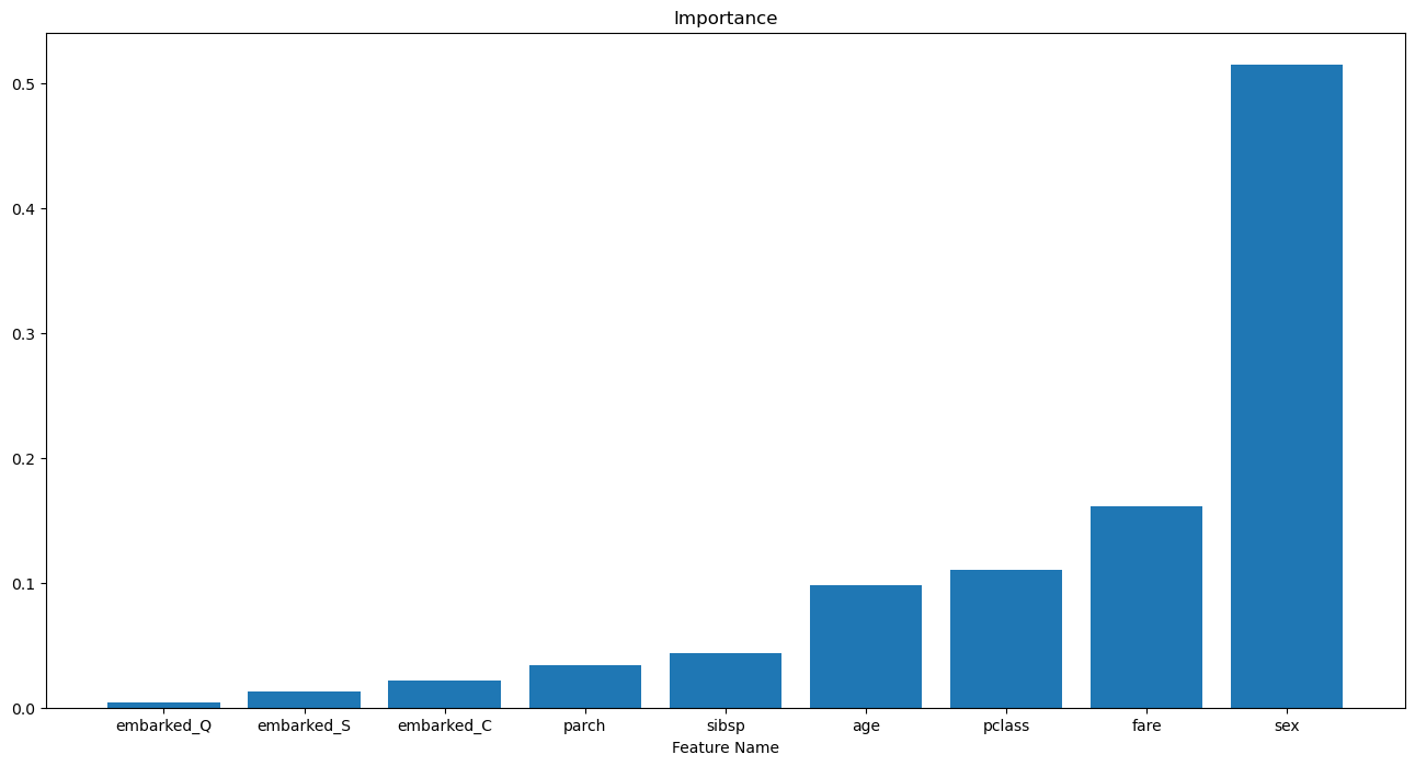
../../../../_images/38275ca38008f22a7838d06772d0a0ed7d336f9647dee9f5acdd5249aa5ad397.png

(?) Do we need all 3: embarked_C, embarked_Q and embarked_S? Look at the options of get_dummies().

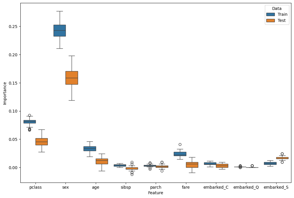
Permutation Effect#

This is a more general method to measure the importance of a feature.
We basically replace the values with “noise” to see how much performance has been deteriorated.

(#) The SciKit Learn’s function which automates the process is permutation_importance().
(#) This is highly time consuming operation. Hence the speed of decision trees based methods creates a synergy.
(#) The importance is strongly linked to the estimator in use.

# Test Permutations
oFeatImpPermTrain = permutation_importance(oRndForestsCls, dfXTrain, dsYTrain, n_repeats = numRepeats)
oFeatImpPermTest  = permutation_importance(oRndForestsCls, dfXTest, dsYTest, n_repeats = numRepeats)

# Generate Data Frame

dT = {'Feature': [], 'Importance': [], 'Data': []}

for (dataName, mScore) in [('Train', oFeatImpPermTrain.importances), ('Test', oFeatImpPermTest.importances)]:
    for ii, featName in enumerate(dfX.columns):
        for jj in range(numRepeats):
            dT['Feature'].append(featName)
            dT['Importance'].append(mScore[ii, jj])
            dT['Data'].append(dataName)

dfFeatImpPerm = pd.DataFrame(dT)
dfFeatImpPerm

	Feature	Importance	Data
0	pclass	0.078491	Train
1	pclass	0.075433	Train
2	pclass	0.076453	Train
3	pclass	0.089704	Train
4	pclass	0.082569	Train
...	...	...	...
895	embarked_S	0.021341	Test
896	embarked_S	0.018293	Test
897	embarked_S	0.018293	Test
898	embarked_S	0.015244	Test
899	embarked_S	0.018293	Test

900 rows × 3 columns

# Plot Results
hF, hA = plt.subplots(figsize = (12, 8))
sns.boxplot(data = dfFeatImpPerm, x = 'Feature', y = 'Importance', hue = 'Data', ax = hA)

plt.show()

../../../../_images/456ebe869093aa63adb98028616d6f8b5a774dbc9bcc50f3337e081adc070481.png

(@) Try extracting better results by using the dropped features.