Non Separable Problem#
Non-Separable Problems in Machine Learning#
In machine learning, a non-separable problem refers to a situation where the data points of different classes cannot be separated by a single linear decision boundary. One classic example of such a problem is the XOR problem.
The XOR Problem#
The XOR (exclusive OR) problem is a fundamental example of a non-linearly separable problem. It involves a binary classification task where the inputs and outputs are as follows:
Inputs: (0, 0) -> Output: 0
Inputs: (0, 1) -> Output: 1
Inputs: (1, 0) -> Output: 1
Inputs: (1, 1) -> Output: 0
If you plot these points on a 2D plane, you will find that there is no straight line that can separate the points of class 0 from the points of class 1.
Mapping to a Higher Dimensional Space#
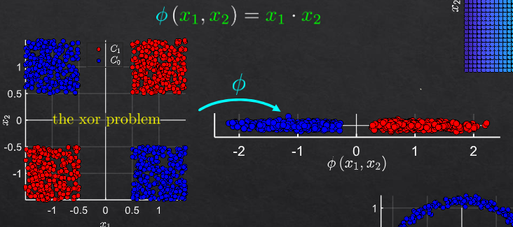
To solve non-separable problems like the XOR problem, we can use a technique known as feature mapping. This involves transforming the original input space into a higher-dimensional space where the problem becomes linearly separable.
For the XOR problem, one effective feature mapping is:
\( z_1 = x_1 \)
\( z_2 = x_2 \)
\( z_3 = x_1 \cdot x_2 \)
By adding the third feature \( z_3 \), the problem can now be linearly separable in the 3D space.
\( (0, 0) \) becomes \( (0, 0, 0) \)
\( (0, 1) \) becomes \( (0, 1, 0) \)
\( (1, 0) \) becomes \( (1, 0, 0) \)
\( (1, 1) \) becomes \( (1, 1, 1) \)
In this 3D space, we can separate the points using a linear plane, making the problem solvable with a linear classifier.
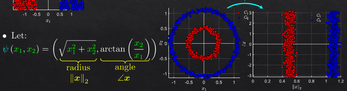
Example 2: Radial Basis Function (RBF)#
Another common transformation technique is the use of Radial Basis Functions (RBF). This is particularly useful for data that is not linearly separable in its original space but can be separated in a transformed space. The RBF is defined as:
where \( \gamma \) is a parameter that controls the width of the RBF, and \( c \) is the center of the function.
Example:
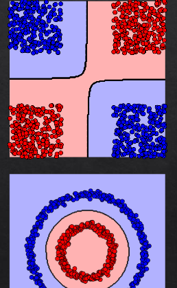
Imagine a simple 2D dataset with a circular decision boundary:
Points inside the circle belong to class 0.
Points outside the circle belong to class 1.
In the original 2D space, these points cannot be separated by a linear decision boundary. However, by applying an RBF transformation, we can map these points to a higher-dimensional space where a linear separation is possible.
Returning to the Original Domain#
After mapping the data to a higher-dimensional space and applying a linear classifier, the classification results can be translated back to the original space. This process involves using the same mapping functions that were applied initially. In practice, this means that once we have trained our model in the transformed space, we can apply the model to new data points by first transforming them and then applying the learned linear decision boundary.
feature transformation#
example1
example2
return to original domain#
we will train linear classifier in the new domain
but to see the original domain separator: calc each point to decide in which class it belongs