MultiDimensional Scaling (MDS)

Notebook by:

• Royi Avital RoyiAvital@fixelalgorithms.com

Revision History

Version	Date	User	Content / Changes
1.0.000	13/04/2024	Royi Avital	First version

# Import Packages

# General Tools
import numpy as np
import scipy as sp
import pandas as pd

# Machine Learning
from sklearn.datasets import make_s_curve
from sklearn.manifold import MDS

# Miscellaneous
import math
import os
from platform import python_version
import random
import timeit

# Typing
from typing import Callable, Dict, List, Optional, Self, Set, Tuple, Union

# Visualization
import matplotlib as mpl
import matplotlib.pyplot as plt
import seaborn as sns

# Jupyter
from IPython import get_ipython
from IPython.display import Image
from IPython.display import display
from ipywidgets import Dropdown, FloatSlider, interact, IntSlider, Layout, SelectionSlider
from ipywidgets import interact

Notations

• (?) Question to answer interactively.

• (!) Simple task to add code for the notebook.

• (@) Optional / Extra self practice.

• (#) Note / Useful resource / Food for thought.

Code Notations:

someVar    = 2; #<! Notation for a variable
vVector    = np.random.rand(4) #<! Notation for 1D array
mMatrix    = np.random.rand(4, 3) #<! Notation for 2D array
tTensor    = np.random.rand(4, 3, 2, 3) #<! Notation for nD array (Tensor)
tuTuple    = (1, 2, 3) #<! Notation for a tuple
lList      = [1, 2, 3] #<! Notation for a list
dDict      = {1: 3, 2: 2, 3: 1} #<! Notation for a dictionary
oObj       = MyClass() #<! Notation for an object
dfData     = pd.DataFrame() #<! Notation for a data frame
dsData     = pd.Series() #<! Notation for a series
hObj       = plt.Axes() #<! Notation for an object / handler / function handler

Code Exercise

• Single line fill

vallToFill = ???

• Multi Line to Fill (At least one)

# You need to start writing
????

• Section to Fill

#===========================Fill This===========================#
# 1. Explanation about what to do.
# !! Remarks to follow / take under consideration.
mX = ???

???
#===============================================================#

# Configuration
# %matplotlib inline

seedNum = 512
np.random.seed(seedNum)
random.seed(seedNum)

# Matplotlib default color palette
lMatPltLibclr = ['#1f77b4', '#ff7f0e', '#2ca02c', '#d62728', '#9467bd', '#8c564b', '#e377c2', '#7f7f7f', '#bcbd22', '#17becf']
# sns.set_theme() #>! Apply SeaBorn theme

runInGoogleColab = 'google.colab' in str(get_ipython())

# Constants

FIG_SIZE_DEF    = (8, 8)
ELM_SIZE_DEF    = 50
CLASS_COLOR     = ('b', 'r')
EDGE_COLOR      = 'k'
MARKER_SIZE_DEF = 10
LINE_WIDTH_DEF  = 2

# Courses Packages
import sys
sys.path.append('../')
sys.path.append('../../')
sys.path.append('../../../')
from utils.DataVisualization import PlotScatterData, PlotScatterData3D

# General Auxiliary Functions

Dimensionality Reduction by MDS

The MDS is a non linear transformation from \(\mathbb{R}^{D} \to \mathbb{R}^{d}\) where \(d \ll D\).
Given a set \(\mathcal{X} = {\left\{ \boldsymbol{x}_{i} \in \mathbb{R}^{D} \right\}}_{i = 1}^{n}\) is builds the set \(\mathcal{Z} = {\left\{ \boldsymbol{z}_{i} \in \mathbb{R}^{d} \right\}}_{i = 1}^{n}\) such that the distance matrices of each set are similar.

In this notebook:

• We’ll implement the classic MDS.

• We’ll use the data set to show the effects of dimensionality reduction.

# Parameters

# Data
numSamples = 1000

# Model
lowDim = 2

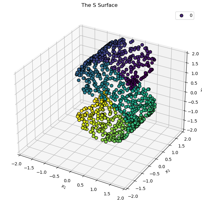
Generate / Load Data

In this notebook we’ll use SciKit Learn’s make_s_curve to generated data.

# Generate Data
mX, vC = make_s_curve(numSamples) #<! Results are random beyond the noise

print(f'The features data shape: {mX.shape}')
print(f'The features data type: {mX.dtype}')

The features data shape: (1000, 3)
The features data type: float64

Plot Data

# Plot the Data

hA = PlotScatterData3D(mX, vC = vC)
hA.set_xlim([-2, 2])
hA.set_ylim([-2, 2])
hA.set_zlim([-2, 2])
hA.set_title('The S Surface')

plt.show()

Applying Dimensionality Reduction - MDS

In this section we’ll implement the Classic MDs:

Non Metric (Classic) MDS

\[\min_{\left\{ \boldsymbol{z}_{i}\in\mathbb{R}^{d}\right\} }\sum_{i=1}^{N}\sum_{j=1}^{N}\left(\boldsymbol{K}_{x}\left[i,j\right]-\left\langle \boldsymbol{z}_{i},\boldsymbol{z}_{j}\right\rangle \right)^{2}\]

1. set \(\boldsymbol{K}_{x}=-\frac{1}{2}\boldsymbol{J}\boldsymbol{D}_{x}\boldsymbol{J}\)
   where \(\boldsymbol{J}=\left(\boldsymbol{I}-\frac{1}{N}\boldsymbol{1}\boldsymbol{1}^{T}\right)\)

2. Decompose \(\boldsymbol{K}_{x}=\boldsymbol{W}\boldsymbol{\Lambda}\boldsymbol{W}\)

3. set \(\boldsymbol{Z}=\boldsymbol{\Lambda}_{d}^{\frac{1}{2}}\boldsymbol{W}_{d}^{T}\)

• (#) The non metric MDS matches (Kernel) PCA.

• (#) It is assumed above that the eigen values matrix \(\boldsymbol{\Lambda}\) is sorted.

• (#) For Euclidean distance there is a closed form solution (As with the PCA).

# Classic MDS Implementation

def ClassicalMDS( mD: np.ndarray, lowDim: int ) -> np.ndarray:
    numSamples = mD.shape[0]

    mJ     = np.eye(numSamples) - ((1 / numSamples) * np.ones((numSamples, numSamples)))
    mK     = -0.5 * mJ @ mD @ mJ #<! Due to the form of mJ one can avoid the matrix multiplication
    vL, mW = np.linalg.eigh(mK)
    
    # Sort Eigen Values
    vIdx   = np.argsort(-vL)
    vL     = vL[vIdx]
    mW     = mW[:, vIdx]
    # Reconstruct
    mZ     = mW[:, :lowDim] * np.sqrt(vL[:lowDim])
    
    return mZ

# Apply the MDS

# Build the Distance Matrix
mD  = sp.spatial.distance.squareform(sp.spatial.distance.pdist(mX))
# The MDS output
mZ1 = ClassicalMDS(np.square(mD), lowDim)

• (?) Could we achieve the above using a different method?

# Plot the Low Dimensional Data

hA = PlotScatterData3D(mZ1, vC = vC, axesProjection = None, figSize = (8, 8))
hA.set_xlabel('${{z}}_{{1}}$')
hA.set_ylabel('${{z}}_{{2}}$')
hA.set_box_aspect(1)
hA.set_title('Classical Euclidean MDS = PCA')

plt.show()

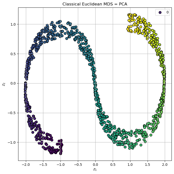
• (#) The Non Metric MDS is guaranteed to keep the order of distances, but not the distance itself.

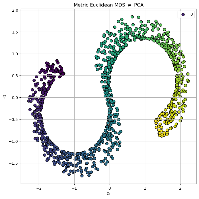
Metric MDS

\[\min_{\left\{ \boldsymbol{z}_{i}\in\mathbb{R}^{d}\right\} }\sum_{i=1}^{N}\sum_{j=1}^{N}\left(d\left(\boldsymbol{x}_{i},\boldsymbol{x}_{j}\right)-\left\Vert \boldsymbol{z}_{i}-\boldsymbol{z}_{j}\right\Vert _{2}\right)^{2}\]

the above is not deterministic (It is a non convex optimization problem)!

# Apply MDS using SciKit Learn

oMdsDr = MDS(n_components = lowDim, dissimilarity = 'precomputed', normalized_stress = 'auto')
mZ2 = oMdsDr.fit_transform(mD)

• (?) Are the results deterministic in the case above?

• (#) The Metric MDS tries to rebuild the data in low dimension with as similar as it can distance matrix. Yet it is not guaranteed to have the same distance.

# Plot the Low Dimensional Data

hA = PlotScatterData3D(mZ2, vC = vC, axesProjection = None, figSize = (8, 8))
hA.set_xlabel('${{z}}_{{1}}$')
hA.set_ylabel('${{z}}_{{2}}$')
hA.set_box_aspect(1)
hA.set_title(r'Metric Euclidean MDS $\neq$ PCA')

plt.show()

Metric MDS with Geodesic Distance

We have access to the geodesic distance using vC, the position along the “main” axis.

# Geodesic Distance

mGeodesicDist = sp.spatial.distance.squareform(sp.spatial.distance.pdist(np.c_[vC, mX[:, 1]]))
mZ3           = oMdsDr.fit_transform(mGeodesicDist)

• (?) Can we use the geodesic distance in real world?

# Plot the Low Dimensional Data

hA = PlotScatterData3D(mZ3, vC = vC, axesProjection = None, figSize = (8, 8))
hA.set_xlabel('${{z}}_{{1}}$')
hA.set_ylabel('${{z}}_{{2}}$')
hA.set_box_aspect(1)
hA.set_title(r'Metric Geodesic MDS $\neq$ PCA')

plt.show()

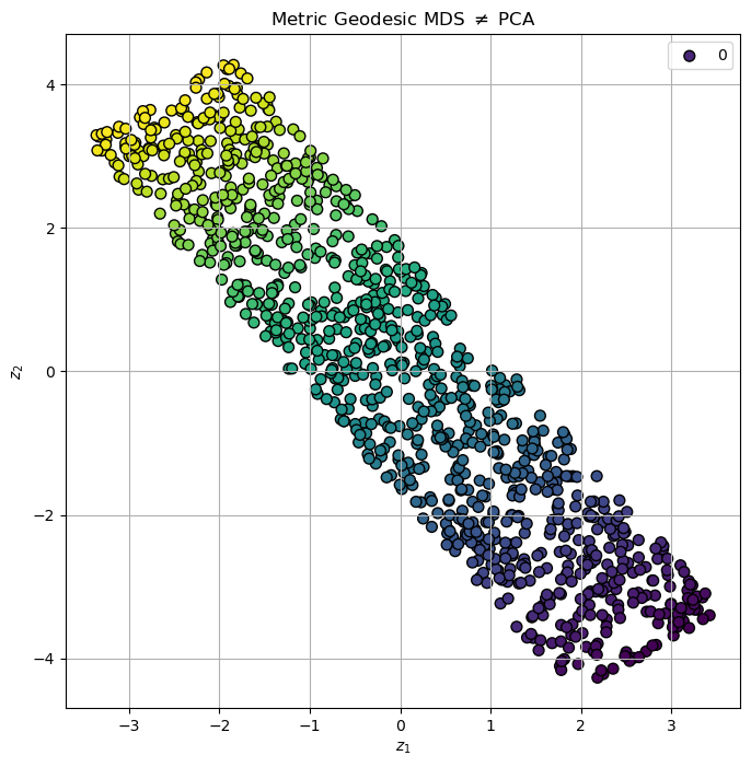
• (?) Is the result above better than the previous ones? Why?