cifar10-2d-convolution#
Image Classification with 2D Convolution (CIFAR 10)#
Notebook by:
Royi Avital RoyiAvital@fixelalgorithms.com
Revision History#
Version |
Date |
User |
Content / Changes |
|---|---|---|---|
1.0.000 |
27/04/2024 |
Royi Avital |
First version |
![]()
# Import Packages

# General Tools
import numpy as np
import scipy as sp
import pandas as pd

# Machine Learning

# Deep Learning
import torch
import torch.nn            as nn
from torch.optim.optimizer import Optimizer
from torch.utils.data import DataLoader
from torch.utils.tensorboard import SummaryWriter
import torchinfo
from torchmetrics.classification import MulticlassAccuracy
import torchvision

# Miscellaneous
import math
import os
from platform import python_version
import random
import time

# Typing
from typing import Callable, Dict, Generator, List, Optional, Self, Set, Tuple, Union

# Visualization
import matplotlib as mpl
import matplotlib.pyplot as plt
import seaborn as sns

# Jupyter
from IPython import get_ipython
from IPython.display import HTML, Image
from IPython.display import display
from ipywidgets import Dropdown, FloatSlider, interact, IntSlider, Layout, SelectionSlider
from ipywidgets import interact
Notations#
(?) Question to answer interactively.
(!) Simple task to add code for the notebook.
(@) Optional / Extra self practice.
(#) Note / Useful resource / Food for thought.
Code Notations:
someVar    = 2; #<! Notation for a variable
vVector    = np.random.rand(4) #<! Notation for 1D array
mMatrix    = np.random.rand(4, 3) #<! Notation for 2D array
tTensor    = np.random.rand(4, 3, 2, 3) #<! Notation for nD array (Tensor)
tuTuple    = (1, 2, 3) #<! Notation for a tuple
lList      = [1, 2, 3] #<! Notation for a list
dDict      = {1: 3, 2: 2, 3: 1} #<! Notation for a dictionary
oObj       = MyClass() #<! Notation for an object
dfData     = pd.DataFrame() #<! Notation for a data frame
dsData     = pd.Series() #<! Notation for a series
hObj       = plt.Axes() #<! Notation for an object / handler / function handler
Code Exercise#
Single line fill
vallToFill = ???
Multi Line to Fill (At least one)
# You need to start writing
????
Section to Fill
#===========================Fill This===========================#
# 1. Explanation about what to do.
# !! Remarks to follow / take under consideration.
mX = ???

???
#===============================================================#
# Configuration
# %matplotlib inline

seedNum = 512
np.random.seed(seedNum)
random.seed(seedNum)

# Matplotlib default color palette
lMatPltLibclr = ['#1f77b4', '#ff7f0e', '#2ca02c', '#d62728', '#9467bd', '#8c564b', '#e377c2', '#7f7f7f', '#bcbd22', '#17becf']
# sns.set_theme() #>! Apply SeaBorn theme

runInGoogleColab = 'google.colab' in str(get_ipython())

# Improve performance by benchmarking
torch.backends.cudnn.benchmark = True

# Reproducibility
# torch.manual_seed(seedNum)
# torch.backends.cudnn.deterministic = True
# torch.backends.cudnn.benchmark     = False
# Constants

FIG_SIZE_DEF    = (8, 8)
ELM_SIZE_DEF    = 50
CLASS_COLOR     = ('b', 'r')
EDGE_COLOR      = 'k'
MARKER_SIZE_DEF = 10
LINE_WIDTH_DEF  = 2

D_CLASSES_CIFAR_10  = {0: 'Airplane', 1: 'Automobile', 2: 'Bird', 3: 'Cat', 4: 'Deer', 5: 'Dog', 6: 'Frog', 7: 'Horse', 8: 'Ship', 9: 'Truck'}
L_CLASSES_CIFAR_10  = ['Airplane', 'Automobile', 'Bird', 'Cat', 'Deer', 'Dog', 'Frog', 'Horse', 'Ship', 'Truck']
T_IMG_SIZE_CIFAR_10 = (32, 32, 3)

DATA_FOLDER_PATH = 'Data'
# Download Auxiliary Modules for Google Colab
if runInGoogleColab:
    !wget https://raw.githubusercontent.com/FixelAlgorithmsTeam/FixelCourses/master/AIProgram/2024_02/DataManipulation.py
    !wget https://raw.githubusercontent.com/FixelAlgorithmsTeam/FixelCourses/master/AIProgram/2024_02/DataVisualization.py
    !wget https://raw.githubusercontent.com/FixelAlgorithmsTeam/FixelCourses/master/AIProgram/2024_02/DeepLearningPyTorch.py
# Courses Packages
import sys,os
sys.path.append('/home/vlad/utils')
from DataVisualization import PlotLabelsHistogram, PlotMnistImages
from DeepLearningPyTorch import NNMode, TrainModel
# General Auxiliary Functions

def AccuracyLogits( mScore: torch.Tensor, vY: torch.Tensor) -> float:

    vHatY = torch.argmax(mScore.detach(), dim = 1) #<! Logits -> Index (As SoftMax is monotonic)
    valAcc = torch.mean((vHatY == vY).float()).item()

    return valAcc
CIFAR 10 Image Classification with 2D Convolution Net#
This notebook shows the use of Conv2d layer.
The 2D Convolution layer means there are 2 degrees of freedom for the kernel movement.
This notebook applies image classification (Single label per image) on the CIFAR 10 dataset.
The notebook presents:
Building a 2D convolution based model which fits Computer Vision tasks.
Use of
torch.nn.Conv2d.Use of
torch.nn.BatchNorm2d.
(#) Convolution is a Linear Shift Invariant (LSI) operator. Hence it fits the task of processing and extracting features from images.
(#) While the convolution layer is LSI the whole net is not fue to Pool Layers,
(#) One technique to make CNN not sensitive to shifts is by training it on a shifted data set.
(#) Modern CNN’s are commonly attributed to Yan LeCun.
Yet, The first documented CNN is called Neocognitron and attributed to Kunihiko Fukushima.(#) For history see Annotated History of Modern AI and Deep Learning (ArXiV Paper).
# Parameters

# Data

# Model
dropP = 0.2 #<! Dropout Layer

# Training
batchSize   = 256
numWork     = 2 #<! Number of workers
nEpochs     = 30

# Visualization
numImg = 3
Generate / Load Data#
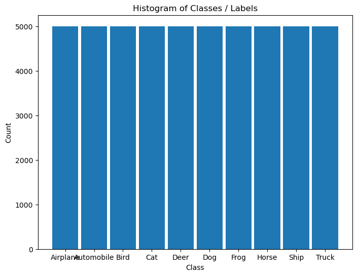
Load the CIFAR 10 Data Set.
It is composed of 60,000 RGB images of size 32x32 with 10 classes uniformly spread.
(#) The dataset is retrieved using Torch Vision’s built in datasets.
# Load Data

# PyTorch
dsTrain = torchvision.datasets.CIFAR10(root = DATA_FOLDER_PATH, train = True,  download = True, transform = torchvision.transforms.ToTensor())
dsTest  = torchvision.datasets.CIFAR10(root = DATA_FOLDER_PATH, train = False, download = True, transform = torchvision.transforms.ToTensor())
lClasses  = dsTrain.classes


print(f'The training data set data shape: {dsTrain.data.shape}')
print(f'The test data set data shape: {dsTest.data.shape}')
print(f'The unique values of the labels: {np.unique(lClasses)}')
Files already downloaded and verified
Files already downloaded and verified
The training data set data shape: (50000, 32, 32, 3)
The test data set data shape: (10000, 32, 32, 3)
The unique values of the labels: ['airplane' 'automobile' 'bird' 'cat' 'deer' 'dog' 'frog' 'horse' 'ship'
 'truck']
(#) The dataset is indexible (Subscriptable). It returns a tuple of the features and the label.
(#) While data is arranged as
H x W x Cthe transformer, when accessing the data, will convert it intoC x H x W.(#) Data arrangement:
(#) PyTorch worked on supporting
NxHxWxC: (Beta) Channels Last Memory Format in PyTorch.
# Element of the Data Set

mX, valY = dsTrain[0]

print(f'The features shape: {mX.shape}')
print(f'The label value: {valY}')
The features shape: torch.Size([3, 32, 32])
The label value: 6
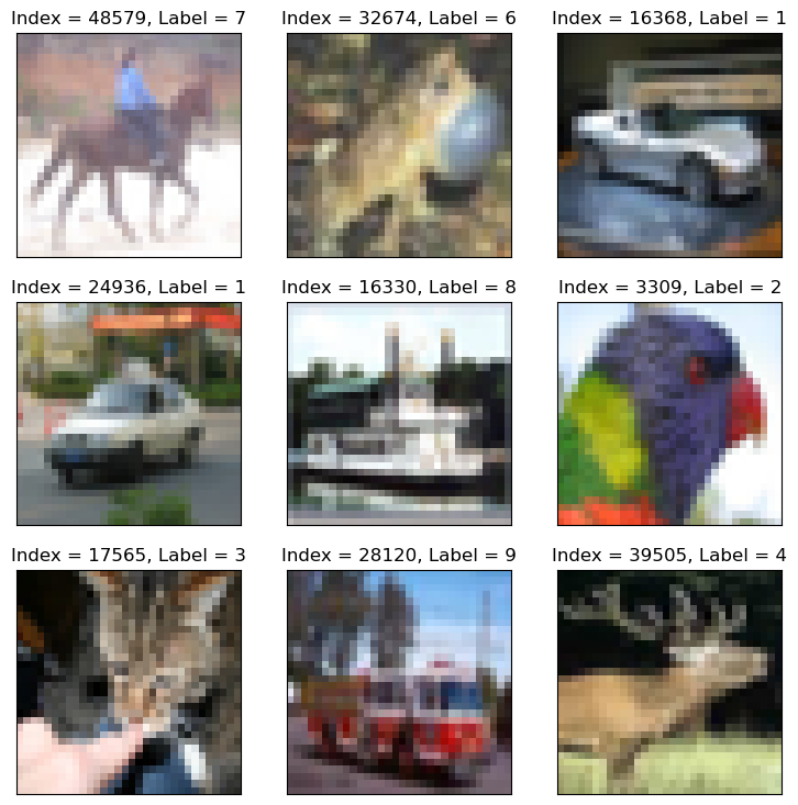
Plot the Data#
# Extract Data

tX = dsTrain.data #<! NumPy Tensor (NDarray)
mX = np.reshape(tX, (tX.shape[0], -1))
vY = dsTrain.targets #<! NumPy Vector
# Plot the Data

hF = PlotMnistImages(mX, vY, numImg, tuImgSize = T_IMG_SIZE_CIFAR_10)
# Histogram of Labels

hA = PlotLabelsHistogram(vY, lClass = L_CLASSES_CIFAR_10)
plt.show()
Pre Process Data#
This section normalizes the data to have zero mean and unit variance per channel.
It is required to calculate:
The average pixel value per channel.
The standard deviation per channel.
# Calculate the Standardization Parameters
vMean = np.mean(dsTrain.data / 255.0, axis = (0, 1, 2))
vStd  = np.std(dsTest.data / 255.0, axis = (0, 1, 2))

print('µ =', vMean)
print('σ =', vStd)
µ = [0.49139968 0.48215841 0.44653091]
σ = [0.24665252 0.24289226 0.26159238]
# Update Transformer

oDataTrns = torchvision.transforms.Compose([       #<! Chaining transformations
    torchvision.transforms.ToTensor(),             #<! Convert to Tensor (C x H x W), Normalizes into [0, 1] (https://pytorch.org/vision/main/generated/torchvision.transforms.ToTensor.html)
    torchvision.transforms.Normalize(vMean, vStd), #<! Normalizes the Data (https://pytorch.org/vision/main/generated/torchvision.transforms.Normalize.html)
    ])

# Update the DS transformer
dsTrain.transform = oDataTrns
dsTest.transform  = oDataTrns
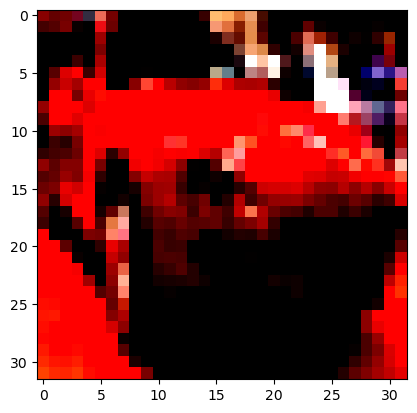
# "Normalized" Image

mX, valY = dsTrain[5]
print(f'mx shape: {mX.shape}')
hF, hA = plt.subplots()
hA.imshow(np.transpose(mX, (1, 2, 0)))
plt.show()
Clipping input data to the valid range for imshow with RGB data ([0..1] for floats or [0..255] for integers).
mx shape: torch.Size([3, 32, 32])
Data Loaders#
The dataloader is the functionality which loads the data into memory in batches.
Its challenge is to bring data fast enough so the Hard Disk is not the training bottleneck.
In order to achieve that, Multi Threading / Multi Process is used.
(#) The multi process, by the
num_workersparameter is not working well out of the box on Windows.
See Errors When Usingnum_workers > 0inDataLoader, On WindowsDataLoaderwithnum_workers > 0Is Slow.
A way to overcome it is to define the training loop as a function in a different module (File) and import it (https://discuss.pytorch.org/t/97564/4, https://discuss.pytorch.org/t/121588/21).(#) The
num_workersshould be set to the lowest number which feeds the GPU fast enough.
The idea is preserve as much as CPU resources to other tasks.(#) On Windows keep the
persistent_workersparameter toTrue(Windows is slower on forking processes / threads).(#) The Dataloader is a generator which can be looped on.
(#) In order to make it iterable it has to be wrapped with
iter().
# Data Loader

dlTrain  = torch.utils.data.DataLoader(dsTrain, shuffle = True, batch_size = 1 * batchSize, num_workers = numWork, persistent_workers = True)
dlTest   = torch.utils.data.DataLoader(dsTest, shuffle = False, batch_size = 2 * batchSize, num_workers = numWork, persistent_workers = True)
(?) Why is the size of the batch twice as big for the test dataset?
# Iterate on the Loader
# The first batch.
tX, vY = next(iter(dlTrain)) #<! PyTorch Tensors

print(f'The batch features dimensions: {tX.shape}')
print(f'The batch labels dimensions: {vY.shape}')
The batch features dimensions: torch.Size([256, 3, 32, 32])
The batch labels dimensions: torch.Size([256])
# Looping
for ii, (tX, vY) in zip(range(1), dlTest): #<! https://stackoverflow.com/questions/36106712
    print(f'The batch features dimensions: {tX.shape}')     ## batch size will be 2 * batchSize
    print(f'The batch labels dimensions: {vY.shape}')
The batch features dimensions: torch.Size([512, 3, 32, 32])
The batch labels dimensions: torch.Size([512])
Define the Model#
The model is defined as a sequential model.
# Model
# Defining a sequential model.

numFeatures = np.prod(tX.shape[1:])

oModel = nn.Sequential(
        nn.Identity(),

        nn.Conv2d(in_channels = 3, out_channels = 30, kernel_size = 3, bias = False),   ## batch false due to use of bath normalization
        nn.BatchNorm2d(num_features = 30),
        nn.ReLU(),
        nn.Dropout2d(p = dropP),

        nn.Conv2d(in_channels = 30, out_channels = 60, kernel_size = 3, bias = False),
        nn.MaxPool2d(kernel_size = 2),
        nn.BatchNorm2d(num_features = 60),
        nn.ReLU(),
        nn.Dropout2d(p = dropP),

        nn.Conv2d(in_channels = 60,  out_channels = 120, kernel_size = 3, bias = False),
        nn.BatchNorm2d(num_features = 120),
        nn.ReLU(),
        nn.Dropout2d(p = dropP),

        nn.Conv2d(in_channels = 120, out_channels = 240, kernel_size = 3, bias = False),
        nn.BatchNorm2d(num_features = 240),
        nn.ReLU(),
        nn.Dropout2d(p = dropP),

        nn.Conv2d(in_channels = 240, out_channels = 500, kernel_size = 3, bias = False),
        nn.MaxPool2d(kernel_size = 2),
        nn.BatchNorm2d(num_features = 500),
        nn.ReLU(),

        nn.AdaptiveAvgPool2d(1),
        nn.Flatten(),
        nn.Linear(500, len(L_CLASSES_CIFAR_10)),
    )

torchinfo.summary(oModel, tX.shape, col_names = ['kernel_size', 'output_size', 'num_params'], device = 'cpu') #<! Added `kernel_size`
===================================================================================================================
Layer (type:depth-idx)                   Kernel Shape              Output Shape              Param #
===================================================================================================================
Sequential                               --                        [256, 10]                 --
├─Identity: 1-1                          --                        [256, 3, 32, 32]          --
├─Conv2d: 1-2                            [3, 3]                    [256, 30, 30, 30]         810
├─BatchNorm2d: 1-3                       --                        [256, 30, 30, 30]         60
├─ReLU: 1-4                              --                        [256, 30, 30, 30]         --
├─Dropout2d: 1-5                         --                        [256, 30, 30, 30]         --
├─Conv2d: 1-6                            [3, 3]                    [256, 60, 28, 28]         16,200
├─MaxPool2d: 1-7                         2                         [256, 60, 14, 14]         --
├─BatchNorm2d: 1-8                       --                        [256, 60, 14, 14]         120
├─ReLU: 1-9                              --                        [256, 60, 14, 14]         --
├─Dropout2d: 1-10                        --                        [256, 60, 14, 14]         --
├─Conv2d: 1-11                           [3, 3]                    [256, 120, 12, 12]        64,800
├─BatchNorm2d: 1-12                      --                        [256, 120, 12, 12]        240
├─ReLU: 1-13                             --                        [256, 120, 12, 12]        --
├─Dropout2d: 1-14                        --                        [256, 120, 12, 12]        --
├─Conv2d: 1-15                           [3, 3]                    [256, 240, 10, 10]        259,200
├─BatchNorm2d: 1-16                      --                        [256, 240, 10, 10]        480
├─ReLU: 1-17                             --                        [256, 240, 10, 10]        --
├─Dropout2d: 1-18                        --                        [256, 240, 10, 10]        --
├─Conv2d: 1-19                           [3, 3]                    [256, 500, 8, 8]          1,080,000
├─MaxPool2d: 1-20                        2                         [256, 500, 4, 4]          --
├─BatchNorm2d: 1-21                      --                        [256, 500, 4, 4]          1,000
├─ReLU: 1-22                             --                        [256, 500, 4, 4]          --
├─AdaptiveAvgPool2d: 1-23                --                        [256, 500, 1, 1]          --
├─Flatten: 1-24                          --                        [256, 500]                --
├─Linear: 1-25                           --                        [256, 10]                 5,010
===================================================================================================================
Total params: 1,427,920
Trainable params: 1,427,920
Non-trainable params: 0
Total mult-adds (Units.GIGABYTES): 30.16
===================================================================================================================
Input size (MB): 3.15
Forward/backward pass size (MB): 482.04
Params size (MB): 5.71
Estimated Total Size (MB): 490.90
===================================================================================================================
(?) Why
in_channels = 3?(?) Why
bias = Falsein the convolution layers?(?) Could the Batch Normalization layer be at the model’s beginning as an alternative to data normalization?
(?) What’s the largest kernel size for
Conv2dto be used after the lastMaxPool2dlayer?(#) BN’s
num_featuresis required to know the number of parameters of the layer.(#) For videos or other 4D dimensions data one could employ
Conv3d.(#) Guideline: The smaller the image gets, the deeper it is (More channels).
The intuition, the beginning of the model learns low level features (Small number), deeper learns combinations of features (Larger number).
# Run Model
# Apply a test run.

tX      = torch.randn(128, 3, 32, 32)
mLogits = oModel(tX) #<! Logit -> Prior to Sigmoid

print(f'The input dimensions: {tX.shape}')
print(f'The output (Logits) dimensions: {mLogits.shape}')
The input dimensions: torch.Size([128, 3, 32, 32])
The output (Logits) dimensions: torch.Size([128, 10])
(#) The Logit Function is the inverse of the Sigmoid Function.
It is commonly used to describe values in the range \(\left( - \infty, \infty \right)\) which can be transformed into probabilities.
Training Loop#
Train the Model#
# Check GPU Availability

runDevice   = torch.device('cuda:0' if torch.cuda.is_available() else 'cpu') #<! The 1st CUDA device
oModel      = oModel.to(runDevice) #<! Transfer model to device
# Set the Loss & Score

hL = nn.CrossEntropyLoss()
hS = MulticlassAccuracy(num_classes = len(L_CLASSES_CIFAR_10), average = 'micro') #<! See documentation for `macro` vs. `micro`
hS = hS.to(runDevice)
(!) Go through
AccuracyLogits()as equivalent tpmicromode.
# Define Optimizer

oOpt = torch.optim.AdamW(oModel.parameters(), lr = 1e-3, betas = (0.9, 0.99), weight_decay = 1e-3) #<! Define optimizer
# Train the Model
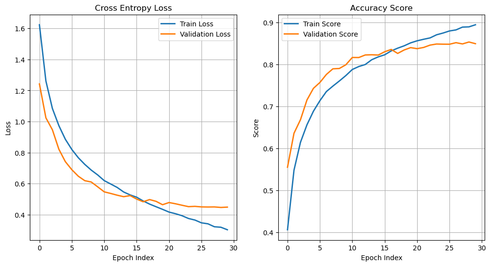
oRunModel, lTrainLoss, lTrainScore, lValLoss, lValScore , _= TrainModel(oModel, dlTrain, dlTest, oOpt, nEpochs, hL, hS)
Epoch    1 / 30 | Train Loss:  1.624 | Val Loss:  1.242 | Train Score:  0.406 | Val Score:  0.555 | Epoch Time: 25.83 | <-- Checkpoint! |
Epoch    2 / 30 | Train Loss:  1.261 | Val Loss:  1.024 | Train Score:  0.548 | Val Score:  0.636 | Epoch Time: 13.48 | <-- Checkpoint! |
Epoch    3 / 30 | Train Loss:  1.084 | Val Loss:  0.947 | Train Score:  0.615 | Val Score:  0.668 | Epoch Time: 12.63 | <-- Checkpoint! |
Epoch    4 / 30 | Train Loss:  0.974 | Val Loss:  0.821 | Train Score:  0.656 | Val Score:  0.715 | Epoch Time: 12.91 | <-- Checkpoint! |
Epoch    5 / 30 | Train Loss:  0.886 | Val Loss:  0.741 | Train Score:  0.689 | Val Score:  0.743 | Epoch Time: 12.56 | <-- Checkpoint! |
Epoch    6 / 30 | Train Loss:  0.820 | Val Loss:  0.690 | Train Score:  0.714 | Val Score:  0.757 | Epoch Time: 12.56 | <-- Checkpoint! |
Epoch    7 / 30 | Train Loss:  0.767 | Val Loss:  0.648 | Train Score:  0.736 | Val Score:  0.776 | Epoch Time: 12.58 | <-- Checkpoint! |
Epoch    8 / 30 | Train Loss:  0.724 | Val Loss:  0.619 | Train Score:  0.749 | Val Score:  0.790 | Epoch Time: 13.58 | <-- Checkpoint! |
Epoch    9 / 30 | Train Loss:  0.687 | Val Loss:  0.610 | Train Score:  0.761 | Val Score:  0.790 | Epoch Time: 14.05 | <-- Checkpoint! |
Epoch   10 / 30 | Train Loss:  0.656 | Val Loss:  0.579 | Train Score:  0.774 | Val Score:  0.799 | Epoch Time: 13.22 | <-- Checkpoint! |
Epoch   11 / 30 | Train Loss:  0.619 | Val Loss:  0.547 | Train Score:  0.788 | Val Score:  0.817 | Epoch Time: 13.76 | <-- Checkpoint! |
Epoch   12 / 30 | Train Loss:  0.597 | Val Loss:  0.536 | Train Score:  0.795 | Val Score:  0.817 | Epoch Time: 14.47 |
Epoch   13 / 30 | Train Loss:  0.575 | Val Loss:  0.525 | Train Score:  0.800 | Val Score:  0.823 | Epoch Time: 13.38 | <-- Checkpoint! |
Epoch   14 / 30 | Train Loss:  0.546 | Val Loss:  0.516 | Train Score:  0.811 | Val Score:  0.823 | Epoch Time: 19.61 | <-- Checkpoint! |
Epoch   15 / 30 | Train Loss:  0.527 | Val Loss:  0.523 | Train Score:  0.818 | Val Score:  0.823 | Epoch Time: 13.13 |
Epoch   16 / 30 | Train Loss:  0.512 | Val Loss:  0.500 | Train Score:  0.823 | Val Score:  0.830 | Epoch Time: 12.85 | <-- Checkpoint! |
Epoch   17 / 30 | Train Loss:  0.488 | Val Loss:  0.483 | Train Score:  0.832 | Val Score:  0.836 | Epoch Time: 12.79 | <-- Checkpoint! |
Epoch   18 / 30 | Train Loss:  0.468 | Val Loss:  0.497 | Train Score:  0.839 | Val Score:  0.826 | Epoch Time: 12.90 |
Epoch   19 / 30 | Train Loss:  0.451 | Val Loss:  0.486 | Train Score:  0.845 | Val Score:  0.835 | Epoch Time: 12.67 |
Epoch   20 / 30 | Train Loss:  0.434 | Val Loss:  0.464 | Train Score:  0.852 | Val Score:  0.840 | Epoch Time: 12.76 | <-- Checkpoint! |
Epoch   21 / 30 | Train Loss:  0.416 | Val Loss:  0.478 | Train Score:  0.856 | Val Score:  0.838 | Epoch Time: 12.69 |
Epoch   22 / 30 | Train Loss:  0.406 | Val Loss:  0.470 | Train Score:  0.860 | Val Score:  0.841 | Epoch Time: 12.69 | <-- Checkpoint! |
Epoch   23 / 30 | Train Loss:  0.393 | Val Loss:  0.461 | Train Score:  0.863 | Val Score:  0.846 | Epoch Time: 12.66 | <-- Checkpoint! |
Epoch   24 / 30 | Train Loss:  0.375 | Val Loss:  0.452 | Train Score:  0.871 | Val Score:  0.849 | Epoch Time: 12.66 | <-- Checkpoint! |
Epoch   25 / 30 | Train Loss:  0.365 | Val Loss:  0.453 | Train Score:  0.875 | Val Score:  0.848 | Epoch Time: 12.68 |
Epoch   26 / 30 | Train Loss:  0.347 | Val Loss:  0.450 | Train Score:  0.880 | Val Score:  0.848 | Epoch Time: 12.65 |
Epoch   27 / 30 | Train Loss:  0.341 | Val Loss:  0.449 | Train Score:  0.882 | Val Score:  0.852 | Epoch Time: 12.67 | <-- Checkpoint! |
Epoch   28 / 30 | Train Loss:  0.322 | Val Loss:  0.450 | Train Score:  0.889 | Val Score:  0.849 | Epoch Time: 12.65 |
Epoch   29 / 30 | Train Loss:  0.319 | Val Loss:  0.446 | Train Score:  0.890 | Val Score:  0.854 | Epoch Time: 12.68 | <-- Checkpoint! |
Epoch   30 / 30 | Train Loss:  0.303 | Val Loss:  0.448 | Train Score:  0.895 | Val Score:  0.850 | Epoch Time: 12.66 |
(?) Why train results are worse than validation for 5-6 epochs?
Results Analysis#
# Plot Results
hF, vHa = plt.subplots(nrows = 1, ncols = 2, figsize = (12, 6))
vHa = vHa.flat

hA = vHa[0]
hA.plot(lTrainLoss, lw = 2, label = 'Train Loss')
hA.plot(lValLoss, lw = 2, label = 'Validation Loss')
hA.grid()
hA.set_title('Cross Entropy Loss')
hA.set_xlabel('Epoch Index')
hA.set_ylabel('Loss')
hA.legend();


hA = vHa[1]
hA.plot(lTrainScore, lw = 2, label = 'Train Score')
hA.plot(lValScore, lw = 2, label = 'Validation Score')
hA.grid()
hA.set_title('Accuracy Score')
hA.set_xlabel('Epoch Index')
hA.set_ylabel('Score')
hA.legend();