
SVM Rand classification#
Notebook by:
Royi Avital RoyiAvital@fixelalgorithms.com
Revision History#
Version |
Date |
User |
Content / Changes |
|---|---|---|---|
1.0.000 |
03/03/2024 |
Royi Avital |
First version |
![]()
# Import Packages

# General Tools
import numpy as np
import scipy as sp
import pandas as pd

# Machine Learning
from sklearn.svm import SVC

# Image Processing

# Machine Learning


# Miscellaneous
import os
from platform import python_version
import random
import timeit

# Typing
from typing import Callable, List, Tuple

# Visualization
import matplotlib as mpl
import matplotlib.pyplot as plt
import seaborn as sns
# from bokeh.plotting import figure, show

# Jupyter
from IPython import get_ipython
from IPython.display import Image, display
from ipywidgets import Dropdown, FloatSlider, interact, IntSlider, Layout
Notations#
(?) Question to answer interactively.
(!) Simple task to add code for the notebook.
(@) Optional / Extra self practice.
(#) Note / Useful resource / Food for thought.
Code Notations:
someVar    = 2; #<! Notation for a variable
vVector    = np.random.rand(4) #<! Notation for 1D array
mMatrix    = np.random.rand(4, 3) #<! Notation for 2D array
tTensor    = np.random.rand(4, 3, 2, 3) #<! Notation for nD array (Tensor)
tuTuple    = (1, 2, 3) #<! Notation for a tuple
lList      = [1, 2, 3] #<! Notation for a list
dDict      = {1: 3, 2: 2, 3: 1} #<! Notation for a dictionary
oObj       = MyClass() #<! Notation for an object
dfData     = pd.DataFrame() #<! Notation for a data frame
dsData     = pd.Series() #<! Notation for a series
hObj       = plt.Axes() #<! Notation for an object / handler / function handler
Code Exercise#
Single line fill
vallToFill = ???
Multi Line to Fill (At least one)
# You need to start writing
????
Section to Fill
#===========================Fill This===========================#
# 1. Explanation about what to do.
# !! Remarks to follow / take under consideration.
mX = ???

???
#===============================================================#
# Configuration
# %matplotlib inline

seedNum = 512
np.random.seed(seedNum)
random.seed(seedNum)

# Matplotlib default color palette
lMatPltLibclr = ['#1f77b4', '#ff7f0e', '#2ca02c', '#d62728', '#9467bd', '#8c564b', '#e377c2', '#7f7f7f', '#bcbd22', '#17becf']
# sns.set_theme() #>! Apply SeaBorn theme

runInGoogleColab = 'google.colab' in str(get_ipython())
# Constants

FIG_SIZE_DEF    = (8, 8)
ELM_SIZE_DEF    = 50
CLASS_COLOR     = ('b', 'r')
EDGE_COLOR      = 'k'
MARKER_SIZE_DEF = 10
LINE_WIDTH_DEF  = 2
# Courses Packages
import sys
sys.path.append('../')
sys.path.append('../../')
sys.path.append('../../../')
from utils.DataVisualization import Plot2DLinearClassifier, PlotBinaryClassData
# General Auxiliary Functions
# Parameters

# Data Generation
numSamples0 = 250
numSamples1 = 250

# Data Visualization
numGridPts = 250
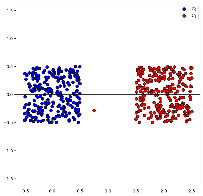
Generate / Load Data#
# Generate Data
numSamples = numSamples0 + numSamples1
mX = np.random.rand(numSamples, 2) - 0.5
mX[numSamples0:, 0] += 2
vY = np.ones((numSamples, ), dtype = np.integer)
vY[:numSamples0] = 0

# One hard sample
mX[0, 0]    = 0.75
vY[0]       = 1

vAxis = np.array([-1, 3, -1, 1])

print(f'The features data shape: {mX.shape}')
print(f'The labels data shape: {vY.shape}')
The features data shape: (500, 2)
The labels data shape: (500,)
Plot the Data#
# Plot the Data
hA = PlotBinaryClassData(mX, vY)
Train a SVM Classifier#
The SciKit Learn Package#
In the course, from now on, we’ll mostly use modules and functions from the SciKit Learn package.
It is mostly known for its API of <model>.fit() and <model>.predict().
This simple choice of convention created the ability to scale in the form of pipelines, chaining models for a greater model.
# Plotting Function

def PlotSVM( C: float ) -> None:
    if C == 0:
        C = 1e-20

    # Train the linear SVM
    oSvmClassifier = SVC(C = C, kernel = 'linear')
    oSvmClassifier = oSvmClassifier.fit(mX, vY)

    # Get model params
    vW =  oSvmClassifier.coef_[0]
    b  = -oSvmClassifier.intercept_

    axisTitle = f'SVM Classifier: $C = {C}$'

    hF, hA = plt.subplots(figsize = (8, 8))
    PlotBinaryClassData(mX, vY, hA = hA, axisTitle = axisTitle)

    vXlim = vAxis[:2]

    hA.plot(vXlim, (b + 1 - vW[0] * vXlim) / vW[1], lw = 2, color = 'orange', ls = '--')
    hA.plot(vXlim, (b + 0 - vW[0] * vXlim) / vW[1], lw = 4, color = 'orange', ls = '-' )
    hA.plot(vXlim, (b - 1 - vW[0] * vXlim) / vW[1], lw = 2, color = 'orange', ls = '--')

    hA.axis(vAxis)
\[ \min_{\boldsymbol{w},b}\frac{1}{2} {\left\| \boldsymbol{w} \right\|}^{2} + C \sum_{i} {\xi}_{i} \]
\[ \xi_{i} := \max \left\{ 0, 1 - {y}_{i} \left( \boldsymbol{w}^{T} \boldsymbol{x}_{i} - b \right) \right\} \]
# Display the Geometry of the Classifier

cSlider = FloatSlider(min = 0, max = 100, step = 1, value = 1, layout = Layout(width = '30%'))
interact(PlotSVM, C = cSlider)

plt.show()
(?) How should
Cchanged with the number of samples?