Kernel PCA#
Kernel Principal Component Analysis (Kernel PCA) is a non-linear extension of Principal Component Analysis (PCA) using techniques of kernel methods. Instead of performing PCA in the original feature space, Kernel PCA allows us to perform PCA in a higher-dimensional feature space implicitly defined by a kernel function. This enables the method to capture non-linear structures in the data.
Overview#
Kernel PCA involves the following steps:
Choose a Kernel Function: Select a kernel function to map the input space to a higher-dimensional feature space.
Compute the Kernel Matrix: Calculate the kernel matrix \( K \) for the input data.
Center the Kernel Matrix: Adjust the kernel matrix to ensure it is centered.
Eigenvalue Decomposition: Perform eigenvalue decomposition on the centered kernel matrix.
Project Data: Use the eigenvectors corresponding to the largest eigenvalues to project the data into the principal component space.
Mathematically, the kernel matrix \( K \) is defined as: $\( K_{ij} = k(\mathbf{x}_i, \mathbf{x}_j) \)\( where \) k(\cdot, \cdot) $ is the chosen kernel function.
Common Kernel Functions#
Polynomial Kernel#
The polynomial kernel is given by: $\( k(\mathbf{x}_i, \mathbf{x}_j) = (\mathbf{x}_i \cdot \mathbf{x}_j + c)^d \)\( where \) d \( is the degree of the polynomial and \) c $ is a constant.
Gaussian (RBF) Kernel#
The Gaussian kernel, also known as the Radial Basis Function (RBF) kernel, is defined as: $\( k(\mathbf{x}_i, \mathbf{x}_j) = \exp \left( -\frac{\|\mathbf{x}_i - \mathbf{x}_j\|^2}{2\sigma^2} \right) \)\( where \) \sigma $ is the bandwidth parameter.
Laplacian Kernel#
The Laplacian kernel is similar to the Gaussian kernel but uses the \( L1 \) norm: $\( k(\mathbf{x}_i, \mathbf{x}_j) = \exp \left( -\frac{\|\mathbf{x}_i - \mathbf{x}_j\|_1}{\sigma} \right) \)\( where \) \sigma $ is the bandwidth parameter.
Sigmoid Kernel#
The sigmoid kernel is given by: $\( k(\mathbf{x}_i, \mathbf{x}_j) = \tanh(\alpha \mathbf{x}_i \cdot \mathbf{x}_j + c) \)\( where \) \alpha \( and \) c $ are kernel parameters.
Real-World Example#
Let’s consider a real-world example where Kernel PCA can be applied. Suppose we have a dataset containing images of handwritten digits (e.g., the MNIST dataset). The digits are represented as pixel intensities in a 2D grid. Linear PCA might not capture the complex, non-linear variations in the handwriting. By applying Kernel PCA with a Gaussian kernel, we can project the data into a higher-dimensional space where these variations are more easily captured, leading to better feature extraction and dimensionality reduction.
Python Implementation#
Here is a brief implementation of Kernel PCA using the Gaussian kernel in Python with the help of the scikit-learn library:
from sklearn.decomposition import KernelPCA
from sklearn.datasets import load_digits
import matplotlib.pyplot as plt

# Load dataset
digits = load_digits()
X = digits.data

# Apply Kernel PCA
kpca = KernelPCA(n_components=2, kernel='rbf', gamma=0.04)
X_kpca = kpca.fit_transform(X)

# Plot the results
plt.scatter(X_kpca[:, 0], X_kpca[:, 1], c=digits.target, cmap='viridis', s=50, alpha=0.7)
plt.colorbar()
plt.title('Kernel PCA on Digits Dataset')
plt.xlabel('Principal Component 1')
plt.ylabel('Principal Component 2')
plt.show()
In this example, we used the Gaussian (RBF) kernel with a bandwidth parameter gamma=0.04 to perform Kernel PCA on the digits dataset. The resulting 2D projection is then visualized using a scatter plot.
Kernel PCA is a powerful technique for capturing non-linear relationships in data, making it useful for a wide range of applications, including image processing, speech recognition, and bioinformatics.
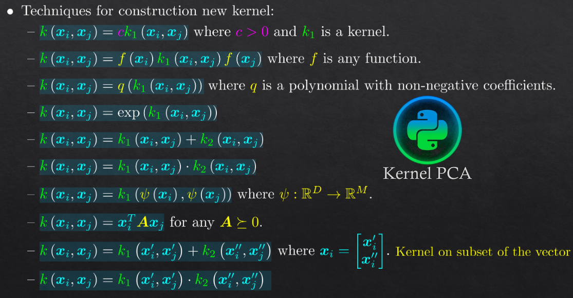
notes#
new kernels#