
ResNet Model#
Notebook by:
Royi Avital RoyiAvital@fixelalgorithms.com
Revision History#
Version |
Date |
User |
Content / Changes |
|---|---|---|---|
1.0.000 |
26/05/2024 |
Royi Avital |
First version |
![]()
# Import Packages

# General Tools
import numpy as np
import scipy as sp
import pandas as pd

# Machine Learning
from sklearn.metrics import confusion_matrix, ConfusionMatrixDisplay
from sklearn.model_selection import ParameterGrid

# Deep Learning
import torch
import torch.nn            as nn
import torch.nn.functional as F
from torch.optim.optimizer import Optimizer
from torch.optim.lr_scheduler import LRScheduler
from torch.utils.data import DataLoader
from torch.utils.tensorboard import SummaryWriter
import torchinfo
from torchmetrics.classification import MulticlassAccuracy
import torchvision
from torchvision.transforms import v2 as TorchVisionTrns

# Miscellaneous
import copy
from enum import auto, Enum, unique
import math
import os
from platform import python_version
import random
import time

# Typing
from typing import Callable, Dict, Generator, List, Optional, Self, Set, Tuple, Union

# Visualization
import matplotlib as mpl
import matplotlib.pyplot as plt
import seaborn as sns

# Jupyter
from IPython import get_ipython
from IPython.display import HTML, Image
from IPython.display import display
from ipywidgets import Dropdown, FloatSlider, interact, IntSlider, Layout, SelectionSlider
from ipywidgets import interact
2024-06-12 06:02:39.873196: I tensorflow/core/platform/cpu_feature_guard.cc:182] This TensorFlow binary is optimized to use available CPU instructions in performance-critical operations.
To enable the following instructions: SSE4.1 SSE4.2 AVX AVX2 FMA, in other operations, rebuild TensorFlow with the appropriate compiler flags.
Notations#
(?) Question to answer interactively.
(!) Simple task to add code for the notebook.
(@) Optional / Extra self practice.
(#) Note / Useful resource / Food for thought.
Code Notations:
someVar    = 2; #<! Notation for a variable
vVector    = np.random.rand(4) #<! Notation for 1D array
mMatrix    = np.random.rand(4, 3) #<! Notation for 2D array
tTensor    = np.random.rand(4, 3, 2, 3) #<! Notation for nD array (Tensor)
tuTuple    = (1, 2, 3) #<! Notation for a tuple
lList      = [1, 2, 3] #<! Notation for a list
dDict      = {1: 3, 2: 2, 3: 1} #<! Notation for a dictionary
oObj       = MyClass() #<! Notation for an object
dfData     = pd.DataFrame() #<! Notation for a data frame
dsData     = pd.Series() #<! Notation for a series
hObj       = plt.Axes() #<! Notation for an object / handler / function handler
Code Exercise#
Single line fill
vallToFill = ???
Multi Line to Fill (At least one)
# You need to start writing
????
Section to Fill
#===========================Fill This===========================#
# 1. Explanation about what to do.
# !! Remarks to follow / take under consideration.
mX = ???

???
#===============================================================#
# Configuration
# %matplotlib inline

seedNum = 512
np.random.seed(seedNum)
random.seed(seedNum)

# Matplotlib default color palette
lMatPltLibclr = ['#1f77b4', '#ff7f0e', '#2ca02c', '#d62728', '#9467bd', '#8c564b', '#e377c2', '#7f7f7f', '#bcbd22', '#17becf']
# sns.set_theme() #>! Apply SeaBorn theme

runInGoogleColab = 'google.colab' in str(get_ipython())

# Improve performance by benchmarking
torch.backends.cudnn.benchmark = True

# Reproducibility (Per PyTorch Version on the same device)
# torch.manual_seed(seedNum)
# torch.backends.cudnn.deterministic = True
# torch.backends.cudnn.benchmark     = False #<! Makes things slower
# Constants

FIG_SIZE_DEF    = (8, 8)
ELM_SIZE_DEF    = 50
CLASS_COLOR     = ('b', 'r')
EDGE_COLOR      = 'k'
MARKER_SIZE_DEF = 10
LINE_WIDTH_DEF  = 2

D_CLASSES_CIFAR_10  = {0: 'Airplane', 1: 'Automobile', 2: 'Bird', 3: 'Cat', 4: 'Deer', 5: 'Dog', 6: 'Frog', 7: 'Horse', 8: 'Ship', 9: 'Truck'}
L_CLASSES_CIFAR_10  = ['Airplane', 'Automobile', 'Bird', 'Cat', 'Deer', 'Dog', 'Frog', 'Horse', 'Ship', 'Truck']
T_IMG_SIZE_CIFAR_10 = (32, 32, 3)

DATA_FOLDER_PATH    = 'Data'
TENSOR_BOARD_BASE   = 'TB'
# Download Auxiliary Modules for Google Colab
if runInGoogleColab:
    !wget https://raw.githubusercontent.com/FixelAlgorithmsTeam/FixelCourses/master/AIProgram/2024_02/DataManipulation.py
    !wget https://raw.githubusercontent.com/FixelAlgorithmsTeam/FixelCourses/master/AIProgram/2024_02/DataVisualization.py
    !wget https://raw.githubusercontent.com/FixelAlgorithmsTeam/FixelCourses/master/AIProgram/2024_02/DeepLearningPyTorch.py
# Courses Packages
import sys
sys.path.append('/home/vlad/utils')
from DataVisualization import PlotLabelsHistogram, PlotMnistImages
from DeepLearningPyTorch import NNMode, ResidualBlock
from DeepLearningPyTorch import InitWeightsKaiNorm, TrainModel
# General Auxiliary Functions
The ResNet Model#
The ResNet model is considered to be one of the most successful architectures.
Its main novelty is the Skip Connection which improved the performance greatly.
By hand waiving the contribution of the skip connection can be explained as:
Learn the Residual
When looking for features, instead of extracting them from the image all needed is to emphasize them.
Namely, as a block, since the input is given, the active path only learns the residual.Ensemble of Models
Since the data can move forward in many paths, one can see each path as a model.Skip Vanishing Gradients
If the gradient is vanishing at a path, the skip connection can skip it during backpropagation.
This notebook presents:
Review a model based on a paper.
Implement the Residual Block.
Implement a ResNet like model.
Train the model on CIFAR10 dataset.
(#) A great recap on ResNet is given in the book Dive into Deep Learning: Residual Networks (ResNet) and ResNeXt.
(#) Analysis of the Skip Connection is given in Skip Connections Eliminate Singularities.
(#) Discussions and notes on skip connection: CrossValidated - Neural Network with Skip Layer Connections, FastAI Forum - What’s the Intuition behind Skip Connections in ResNet.
(#) Intuitive Explanation of Skip Connections in Deep Learning.
# Parameters

# Data
numSamplesPerClsTrain   = 4000
numSamplesPerClsVal     = 400

# Model
dropP = 0.5 #<! Dropout Layer

# Training
batchSize   = 256
numWork     = 2 #<! Number of workers
nEpochs     = 45

# Visualization
numImg = 3
Generate / Load Data#
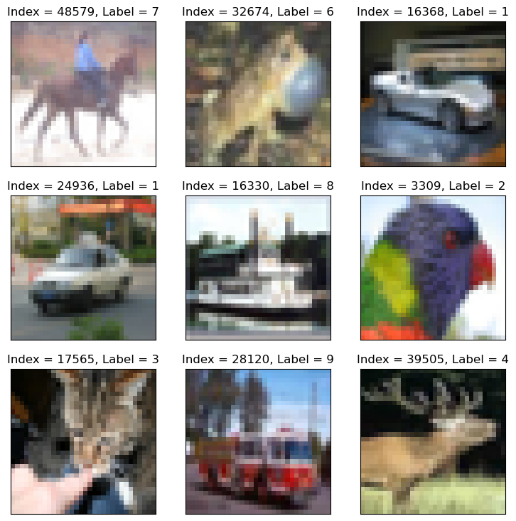
Load the CIFAR 10 Data Set.
It is composed of 60,000 RGB images of size 32x32 with 10 classes uniformly spread.
(#) The dataset is retrieved using Torch Vision’s built in datasets.
# Load Data

dsTrain = torchvision.datasets.CIFAR10(root = DATA_FOLDER_PATH, train = True,  download = True, transform = torchvision.transforms.ToTensor())
dsVal   = torchvision.datasets.CIFAR10(root = DATA_FOLDER_PATH, train = False, download = True, transform = torchvision.transforms.ToTensor())
lClass  = dsTrain.classes


print(f'The training data set data shape: {dsTrain.data.shape}')
print(f'The validation data set data shape: {dsVal.data.shape}')
print(f'The unique values of the labels: {np.unique(lClass)}')
Files already downloaded and verified
Files already downloaded and verified
The training data set data shape: (50000, 32, 32, 3)
The validation data set data shape: (10000, 32, 32, 3)
The unique values of the labels: ['airplane' 'automobile' 'bird' 'cat' 'deer' 'dog' 'frog' 'horse' 'ship'
 'truck']
(#) The dataset is indexible (Subscriptable). It returns a tuple of the features and the label.
(#) While data is arranged as
H x W x Cthe transformer, when accessing the data, will convert it intoC x H x W.
# Element of the Data Set

mX, valY = dsTrain[0]

print(f'The features shape: {mX.shape}')
print(f'The label value: {valY}')
The features shape: torch.Size([3, 32, 32])
The label value: 6
Plot the Data#
# Extract Data

tX = dsTrain.data #<! NumPy Tensor (NDarray)
mX = np.reshape(tX, (tX.shape[0], -1))
vY = dsTrain.targets #<! NumPy Vector
# Plot the Data

hF = PlotMnistImages(mX, vY, numImg, tuImgSize = T_IMG_SIZE_CIFAR_10)
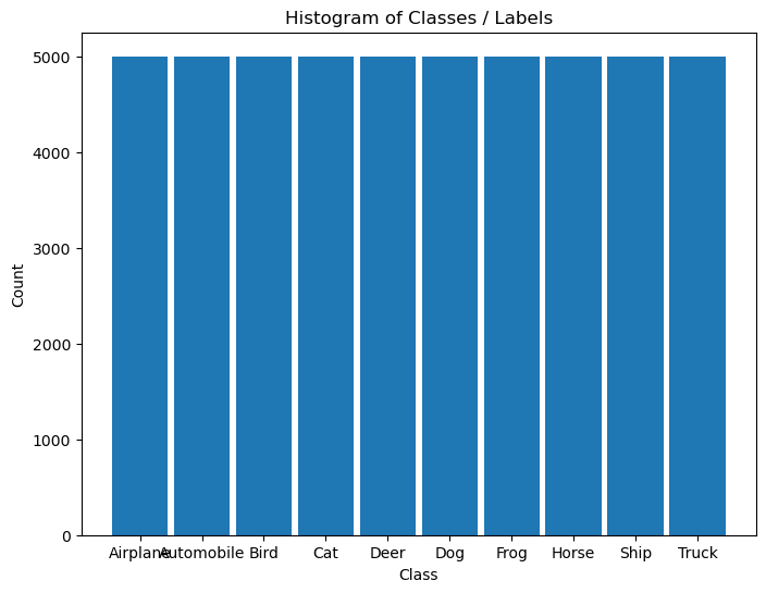
# Histogram of Labels

hA = PlotLabelsHistogram(vY, lClass = L_CLASSES_CIFAR_10)
plt.show()
(?) If data is converted into grayscale, how would it effect the performance of the classifier? Explain.
You may assume the conversion is done using the mean value of the RGB pixel.
Pre Process Data#
This section:
Normalizes the data in a predefined manner.
Takes a sub set of the data.
# Calculate the Standardization Parameters
vMean = np.mean(dsTrain.data / 255.0, axis = (0, 1, 2))
vStd  = np.std(dsVal.data / 255.0, axis = (0, 1, 2))

print('µ =', vMean)
print('σ =', vStd)
µ = [0.49139968 0.48215841 0.44653091]
σ = [0.24665252 0.24289226 0.26159238]
# Update Transforms
# Using v2 Transforms
oDataTrnsTrain = TorchVisionTrns.Compose([
    TorchVisionTrns.ToImage(),
    TorchVisionTrns.ToDtype(torch.float32, scale = True),
    TorchVisionTrns.RandomHorizontalFlip(p = 0.5),
    TorchVisionTrns.Normalize(mean = vMean, std = vStd),
])
oDataTrnsVal = TorchVisionTrns.Compose([
    TorchVisionTrns.ToImage(),
    TorchVisionTrns.ToDtype(torch.float32, scale = True),
    TorchVisionTrns.Normalize(mean = vMean, std = vStd),
])

# Update the DS transformer
dsTrain.transform   = oDataTrnsTrain
dsVal.transform     = oDataTrnsVal
(?) What does
RandomHorizontalFlipdo? Why can it be used?
— we accept the model to know if the image is flipped or not - for real world image why it is helping - it is helping to generalize the model and make the model not be sensitive to the orientation of the image; it is also helping to increase the size of the dataset;
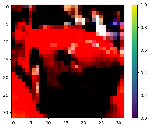
# "Normalized" Image

mX, valY = dsTrain[5]

hF, hA = plt.subplots()
hImg = hA.imshow(np.transpose(mX, (1, 2, 0)))
hF.colorbar(hImg)
plt.show()
Clipping input data to the valid range for imshow with RGB data ([0..1] for floats or [0..255] for integers).
Data Loaders#
This section defines the data loaded.
# Data Loader

dlTrain = torch.utils.data.DataLoader(dsTrain, shuffle = True, batch_size = 1 * batchSize, num_workers = numWork, persistent_workers = True)
dlVal   = torch.utils.data.DataLoader(dsVal, shuffle = False, batch_size = 2 * batchSize, num_workers = numWork, persistent_workers = True)
(?) Why is the size of the batch twice as big for the test dataset?
# Iterate on the Loader
# The first batch.
tX, vY = next(iter(dlTrain)) #<! PyTorch Tensors

print(f'The batch features dimensions: {tX.shape}')
print(f'The batch labels dimensions: {vY.shape}')
The batch features dimensions: torch.Size([256, 3, 32, 32])
The batch labels dimensions: torch.Size([256])
# Looping
for ii, (tX, vY) in zip(range(1), dlVal): #<! https://stackoverflow.com/questions/36106712
    print(f'The batch features dimensions: {tX.shape}')
    print(f'The batch labels dimensions: {vY.shape}')
The batch features dimensions: torch.Size([512, 3, 32, 32])
The batch labels dimensions: torch.Size([512])
Define the Model#
The model is defined as a sequential model built with non sequential blocks.
In PyTorch models are defined by 2 main methods:
The
__init__()Method
Set the parameters and elements of the model.The
forward()Method
Set the structure of the computation.
It holds whether the model is a layer or a sub module of a bigger model.
The Residual Block#
This section implements the residual block as an torch.nn.Module.

(!) Got through the
ResidualBlockclass.(#) The
ResidualBlockclass is an example of a non sequential model (Though it is a block).(#) Some argue that the residual block in the following form yields better results:
nn.Sequential(
            nn.BatchNorm2d(C), nn.ReLU(), nn.Conv2d(C, C, 3, padding = 1, bias = False),
            nn.BatchNorm2d(C), nn.ReLU(), nn.Conv2d(C, C, 3, padding = 1, bias = False)
)
class ResidualBlock( nn.Module ):
    def __init__( self, numChnl: int ) -> None:
        super(ResidualBlock, self).__init__()           // call infra init for all features support

        // define our struct //
        // * the class mode not functional to show better on info graph

        self.oConv2D1       = nn.Conv2d(numChnl, numChnl, kernel_size = 3, padding = 1, bias = False)
                                                                        // pad =1 = to keep the same exit size
        self.oBatchNorm1    = nn.BatchNorm2d(numChnl)
        self.oReLU1         = nn.ReLU(inplace = True)
        self.oConv2D2       = nn.Conv2d(numChnl, numChnl, kernel_size = 3, padding = 1, bias = False)
        self.oBatchNorm2    = nn.BatchNorm2d(numChnl)
        self.oReLU2         = nn.ReLU(inplace = True) #<! No need for it, for better visualization

    def forward( self: Self, tX: torch.Tensor ) -> torch.Tensor:

        tY = self.oReLU1(self.oBatchNorm1(self.oConv2D1(tX)))
        tY = self.oBatchNorm2(self.oConv2D2(tY))
        tY += tX
        tY = self.oReLU2(tY)

        return tY
# The Residual Block
oResBlock = ResidualBlock(64)
torchinfo.summary(oResBlock, (4, 64, 56, 56), col_names = ['kernel_size', 'output_size', 'num_params'], device = 'cpu')
===================================================================================================================
Layer (type:depth-idx)                   Kernel Shape              Output Shape              Param #
===================================================================================================================
ResidualBlock                            --                        [4, 64, 56, 56]           --
├─Conv2d: 1-1                            [3, 3]                    [4, 64, 56, 56]           36,864
├─BatchNorm2d: 1-2                       --                        [4, 64, 56, 56]           128
├─ReLU: 1-3                              --                        [4, 64, 56, 56]           --
├─Conv2d: 1-4                            [3, 3]                    [4, 64, 56, 56]           36,864
├─BatchNorm2d: 1-5                       --                        [4, 64, 56, 56]           128
├─ReLU: 1-6                              --                        [4, 64, 56, 56]           --
===================================================================================================================
Total params: 73,984
Trainable params: 73,984
Non-trainable params: 0
Total mult-adds (Units.MEGABYTES): 924.85
===================================================================================================================
Input size (MB): 3.21
Forward/backward pass size (MB): 25.69
Params size (MB): 0.30
Estimated Total Size (MB): 29.20
===================================================================================================================
(@) Implement the
ResidualBlockclass usingnn.Sequentialto describe the left path.
optional : residul with learned param#
(#) Assume the output of the Residual Layer was \(g \left( \boldsymbol{x} \right) = \alpha f \left( \boldsymbol{x} \right) + \left( 1 - \alpha \right) \boldsymbol{x}\).
If one would like \(\alpha\) to be a learned parameter it would have ot be registered as such.
See PyTorch: Custom nn Modules, Dive into Deep Learning - Builder’s Guide - Custom Layers, Writing a Custom Layer in PyTorch.
class ResidualBlock( nn.Module ):
    def __init__( self, numChnl: int ) -> None:
        super(ResidualBlock, self).__init__()           // call infra init for all features support

        //!!!!

        self.a = torch.nn.Parameter(torch.randn(()))

        //!!!!
        //........
build model#
# Model
# Defining a sequential model.

numChannels = 128

def BuildModel( nC: int ) -> nn.Module:

    oModel = nn.Sequential(
        nn.Identity(),
        nn.Conv2d(3, nC, 3, padding = 1, bias = False),  nn.BatchNorm2d(nC), nn.ReLU(),                  nn.Dropout2d(0.2),
        nn.Conv2d(nC, nC, 3, padding = 1, bias = False), nn.BatchNorm2d(nC), nn.ReLU(), nn.MaxPool2d(2), nn.Dropout2d(0.2),

        ResidualBlock(nC), nn.Dropout2d(0.2),
        ResidualBlock(nC), nn.Dropout2d(0.2),

        nn.AdaptiveAvgPool2d(1),
        nn.Flatten(),
        nn.Linear(nC, 10)
    )

    oModel.apply(InitWeightsKaiNorm)

    return oModel

oModel = BuildModel(numChannels)

torchinfo.summary(oModel, (batchSize, 3, 32, 32), col_names = ['kernel_size', 'output_size', 'num_params'], device = 'cpu')
===================================================================================================================
Layer (type:depth-idx)                   Kernel Shape              Output Shape              Param #
===================================================================================================================
Sequential                               --                        [256, 10]                 --
├─Identity: 1-1                          --                        [256, 3, 32, 32]          --
├─Conv2d: 1-2                            [3, 3]                    [256, 128, 32, 32]        3,456
├─BatchNorm2d: 1-3                       --                        [256, 128, 32, 32]        256
├─ReLU: 1-4                              --                        [256, 128, 32, 32]        --
├─Dropout2d: 1-5                         --                        [256, 128, 32, 32]        --
├─Conv2d: 1-6                            [3, 3]                    [256, 128, 32, 32]        147,456
├─BatchNorm2d: 1-7                       --                        [256, 128, 32, 32]        256
├─ReLU: 1-8                              --                        [256, 128, 32, 32]        --
├─MaxPool2d: 1-9                         2                         [256, 128, 16, 16]        --
├─Dropout2d: 1-10                        --                        [256, 128, 16, 16]        --
├─ResidualBlock: 1-11                    --                        [256, 128, 16, 16]        --
│    └─Conv2d: 2-1                       [3, 3]                    [256, 128, 16, 16]        147,456
│    └─BatchNorm2d: 2-2                  --                        [256, 128, 16, 16]        256
│    └─ReLU: 2-3                         --                        [256, 128, 16, 16]        --
│    └─Conv2d: 2-4                       [3, 3]                    [256, 128, 16, 16]        147,456
│    └─BatchNorm2d: 2-5                  --                        [256, 128, 16, 16]        256
│    └─ReLU: 2-6                         --                        [256, 128, 16, 16]        --
├─Dropout2d: 1-12                        --                        [256, 128, 16, 16]        --
├─ResidualBlock: 1-13                    --                        [256, 128, 16, 16]        --
│    └─Conv2d: 2-7                       [3, 3]                    [256, 128, 16, 16]        147,456
│    └─BatchNorm2d: 2-8                  --                        [256, 128, 16, 16]        256
│    └─ReLU: 2-9                         --                        [256, 128, 16, 16]        --
│    └─Conv2d: 2-10                      [3, 3]                    [256, 128, 16, 16]        147,456
│    └─BatchNorm2d: 2-11                 --                        [256, 128, 16, 16]        256
│    └─ReLU: 2-12                        --                        [256, 128, 16, 16]        --
├─Dropout2d: 1-14                        --                        [256, 128, 16, 16]        --
├─AdaptiveAvgPool2d: 1-15                --                        [256, 128, 1, 1]          --
├─Flatten: 1-16                          --                        [256, 128]                --
├─Linear: 1-17                           --                        [256, 10]                 1,290
===================================================================================================================
Total params: 743,562
Trainable params: 743,562
Non-trainable params: 0
Total mult-adds (Units.GIGABYTES): 78.22
===================================================================================================================
Input size (MB): 3.15
Forward/backward pass size (MB): 1610.63
Params size (MB): 2.97
Estimated Total Size (MB): 1616.75
===================================================================================================================
(@) Use the default initialization and compare results.
(?) What is the motivation to build on your own the ResNet model instead of using the pre trained model?
Think about the dimensions of the dataset samples.
Train the Model#
This section trains the model using different schedulers:
Updates the training function to use more features of TensorBoard.
Trains the model with different hyper parameters.
# Run Device

runDevice = torch.device('cuda:0' if torch.cuda.is_available() else 'cpu') #<! The 1st CUDA device
oModel    = oModel.to(runDevice) #<! Transfer model to device
# Loss and Score Function

hL = nn.CrossEntropyLoss()
hS = MulticlassAccuracy(num_classes = len(lClass), average = 'micro')
hL = hL.to(runDevice) #<! Not required!
hS = hS.to(runDevice)
(#) The averaging mode
macroaverages samples per class and average the result of each class.(#) The averaging mode
microaverages all samples.(?) Given 8 samples of class
Awith 6 predictions being correct and 2 samples of classBwith 1 being correct.
What will be the macro average? What will be the micro average?
A (6/8) =>              macro (75 + 50 ) / 2 = 62.5%
B (1/2) = >             micro 7/10 = 70%

for inbalanced dataset, macro is better ;
# Define Optimizer

oOpt = torch.optim.AdamW(oModel.parameters(), lr = 1e-3, betas = (0.9, 0.99), weight_decay = 1e-3) #<! Define optimizer
# Define Scheduler

oSch = torch.optim.lr_scheduler.OneCycleLR(oOpt, max_lr = 5e-3, total_steps = nEpochs)
# Train Model

oModel, lTrainLoss, lTrainScore, lValLoss, lValScore, lLearnRate = TrainModel(oModel, dlTrain, dlVal, oOpt, nEpochs, hL, hS, oSch = oSch)
Epoch    1 / 45 | Train Loss:  2.248 | Val Loss:  1.666 | Train Score:  0.241 | Val Score:  0.388 | Epoch Time: 34.75 | <-- Checkpoint! |
Epoch    2 / 45 | Train Loss:  1.842 | Val Loss:  1.485 | Train Score:  0.323 | Val Score:  0.465 | Epoch Time: 26.85 | <-- Checkpoint! |
Epoch    3 / 45 | Train Loss:  1.632 | Val Loss:  1.291 | Train Score:  0.396 | Val Score:  0.540 | Epoch Time: 26.50 | <-- Checkpoint! |
Epoch    4 / 45 | Train Loss:  1.423 | Val Loss:  1.148 | Train Score:  0.480 | Val Score:  0.594 | Epoch Time: 26.63 | <-- Checkpoint! |
Epoch    5 / 45 | Train Loss:  1.257 | Val Loss:  1.056 | Train Score:  0.544 | Val Score:  0.622 | Epoch Time: 28.36 | <-- Checkpoint! |
Epoch    6 / 45 | Train Loss:  1.129 | Val Loss:  0.942 | Train Score:  0.596 | Val Score:  0.659 | Epoch Time: 29.49 | <-- Checkpoint! |
Epoch    7 / 45 | Train Loss:  1.024 | Val Loss:  0.876 | Train Score:  0.636 | Val Score:  0.685 | Epoch Time: 28.71 | <-- Checkpoint! |
Epoch    8 / 45 | Train Loss:  0.934 | Val Loss:  0.838 | Train Score:  0.669 | Val Score:  0.702 | Epoch Time: 29.27 | <-- Checkpoint! |
Epoch    9 / 45 | Train Loss:  0.849 | Val Loss:  0.756 | Train Score:  0.700 | Val Score:  0.730 | Epoch Time: 27.51 | <-- Checkpoint! |
Epoch   10 / 45 | Train Loss:  0.771 | Val Loss:  0.639 | Train Score:  0.732 | Val Score:  0.773 | Epoch Time: 27.21 | <-- Checkpoint! |
Epoch   11 / 45 | Train Loss:  0.705 | Val Loss:  0.614 | Train Score:  0.756 | Val Score:  0.790 | Epoch Time: 26.77 | <-- Checkpoint! |
Epoch   12 / 45 | Train Loss:  0.657 | Val Loss:  0.536 | Train Score:  0.774 | Val Score:  0.808 | Epoch Time: 26.79 | <-- Checkpoint! |
Epoch   13 / 45 | Train Loss:  0.607 | Val Loss:  0.535 | Train Score:  0.791 | Val Score:  0.815 | Epoch Time: 26.72 | <-- Checkpoint! |
Epoch   14 / 45 | Train Loss:  0.564 | Val Loss:  0.516 | Train Score:  0.808 | Val Score:  0.828 | Epoch Time: 26.62 | <-- Checkpoint! |
Epoch   15 / 45 | Train Loss:  0.529 | Val Loss:  0.506 | Train Score:  0.818 | Val Score:  0.823 | Epoch Time: 26.76 |
Epoch   16 / 45 | Train Loss:  0.504 | Val Loss:  0.443 | Train Score:  0.827 | Val Score:  0.846 | Epoch Time: 26.64 | <-- Checkpoint! |
Epoch   17 / 45 | Train Loss:  0.475 | Val Loss:  0.422 | Train Score:  0.837 | Val Score:  0.856 | Epoch Time: 26.79 | <-- Checkpoint! |
Epoch   18 / 45 | Train Loss:  0.452 | Val Loss:  0.424 | Train Score:  0.845 | Val Score:  0.857 | Epoch Time: 27.09 | <-- Checkpoint! |
Epoch   19 / 45 | Train Loss:  0.423 | Val Loss:  0.404 | Train Score:  0.855 | Val Score:  0.862 | Epoch Time: 26.67 | <-- Checkpoint! |
Epoch   20 / 45 | Train Loss:  0.408 | Val Loss:  0.412 | Train Score:  0.861 | Val Score:  0.857 | Epoch Time: 26.80 |
Epoch   21 / 45 | Train Loss:  0.388 | Val Loss:  0.406 | Train Score:  0.866 | Val Score:  0.863 | Epoch Time: 26.76 | <-- Checkpoint! |
Epoch   22 / 45 | Train Loss:  0.370 | Val Loss:  0.393 | Train Score:  0.872 | Val Score:  0.872 | Epoch Time: 26.82 | <-- Checkpoint! |
Epoch   23 / 45 | Train Loss:  0.355 | Val Loss:  0.361 | Train Score:  0.878 | Val Score:  0.876 | Epoch Time: 26.86 | <-- Checkpoint! |
Epoch   24 / 45 | Train Loss:  0.341 | Val Loss:  0.360 | Train Score:  0.883 | Val Score:  0.876 | Epoch Time: 26.78 | <-- Checkpoint! |
Epoch   25 / 45 | Train Loss:  0.326 | Val Loss:  0.349 | Train Score:  0.887 | Val Score:  0.882 | Epoch Time: 26.73 | <-- Checkpoint! |
Epoch   26 / 45 | Train Loss:  0.307 | Val Loss:  0.339 | Train Score:  0.895 | Val Score:  0.886 | Epoch Time: 26.72 | <-- Checkpoint! |
Epoch   27 / 45 | Train Loss:  0.295 | Val Loss:  0.338 | Train Score:  0.896 | Val Score:  0.884 | Epoch Time: 26.72 |
Epoch   28 / 45 | Train Loss:  0.279 | Val Loss:  0.334 | Train Score:  0.903 | Val Score:  0.887 | Epoch Time: 26.69 | <-- Checkpoint! |
Epoch   29 / 45 | Train Loss:  0.266 | Val Loss:  0.331 | Train Score:  0.906 | Val Score:  0.889 | Epoch Time: 26.73 | <-- Checkpoint! |
Epoch   30 / 45 | Train Loss:  0.254 | Val Loss:  0.330 | Train Score:  0.912 | Val Score:  0.892 | Epoch Time: 26.74 | <-- Checkpoint! |
Epoch   31 / 45 | Train Loss:  0.237 | Val Loss:  0.325 | Train Score:  0.917 | Val Score:  0.895 | Epoch Time: 26.80 | <-- Checkpoint! |
Epoch   32 / 45 | Train Loss:  0.225 | Val Loss:  0.319 | Train Score:  0.922 | Val Score:  0.896 | Epoch Time: 26.83 | <-- Checkpoint! |
Epoch   33 / 45 | Train Loss:  0.219 | Val Loss:  0.307 | Train Score:  0.923 | Val Score:  0.900 | Epoch Time: 26.85 | <-- Checkpoint! |
Epoch   34 / 45 | Train Loss:  0.210 | Val Loss:  0.309 | Train Score:  0.927 | Val Score:  0.901 | Epoch Time: 26.79 | <-- Checkpoint! |
Epoch   35 / 45 | Train Loss:  0.200 | Val Loss:  0.306 | Train Score:  0.930 | Val Score:  0.898 | Epoch Time: 26.68 |
Epoch   36 / 45 | Train Loss:  0.188 | Val Loss:  0.304 | Train Score:  0.934 | Val Score:  0.900 | Epoch Time: 26.62 |
Epoch   37 / 45 | Train Loss:  0.183 | Val Loss:  0.309 | Train Score:  0.937 | Val Score:  0.899 | Epoch Time: 26.60 |
Epoch   38 / 45 | Train Loss:  0.175 | Val Loss:  0.308 | Train Score:  0.939 | Val Score:  0.900 | Epoch Time: 26.72 |
Epoch   39 / 45 | Train Loss:  0.170 | Val Loss:  0.309 | Train Score:  0.941 | Val Score:  0.900 | Epoch Time: 26.76 |
Epoch   40 / 45 | Train Loss:  0.164 | Val Loss:  0.308 | Train Score:  0.942 | Val Score:  0.901 | Epoch Time: 26.63 |
Epoch   41 / 45 | Train Loss:  0.163 | Val Loss:  0.307 | Train Score:  0.943 | Val Score:  0.901 | Epoch Time: 26.69 | <-- Checkpoint! |
Epoch   42 / 45 | Train Loss:  0.161 | Val Loss:  0.305 | Train Score:  0.944 | Val Score:  0.900 | Epoch Time: 26.71 |
Epoch   43 / 45 | Train Loss:  0.157 | Val Loss:  0.305 | Train Score:  0.946 | Val Score:  0.901 | Epoch Time: 26.65 | <-- Checkpoint! |
Epoch   44 / 45 | Train Loss:  0.156 | Val Loss:  0.306 | Train Score:  0.945 | Val Score:  0.902 | Epoch Time: 26.79 | <-- Checkpoint! |
Epoch   45 / 45 | Train Loss:  0.156 | Val Loss:  0.304 | Train Score:  0.946 | Val Score:  0.902 | Epoch Time: 26.65 | <-- Checkpoint! |
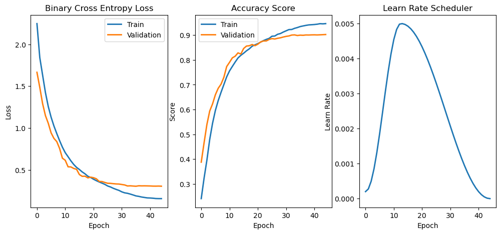
# Plot Training Phase

hF, vHa = plt.subplots(nrows = 1, ncols = 3, figsize = (12, 5))
vHa = np.ravel(vHa)

hA = vHa[0]
hA.plot(lTrainLoss, lw = 2, label = 'Train')
hA.plot(lValLoss, lw = 2, label = 'Validation')
hA.set_title('Binary Cross Entropy Loss')
hA.set_xlabel('Epoch')
hA.set_ylabel('Loss')
hA.legend()

hA = vHa[1]
hA.plot(lTrainScore, lw = 2, label = 'Train')
hA.plot(lValScore, lw = 2, label = 'Validation')
hA.set_title('Accuracy Score')
hA.set_xlabel('Epoch')
hA.set_ylabel('Score')
hA.legend()

hA = vHa[2]
hA.plot(lLearnRate, lw = 2)
hA.set_title('Learn Rate Scheduler')
hA.set_xlabel('Epoch')
hA.set_ylabel('Learn Rate')
Text(0, 0.5, 'Learn Rate')
(!) Implement the ResNeXt like model. Start with the block and embed it into the model.